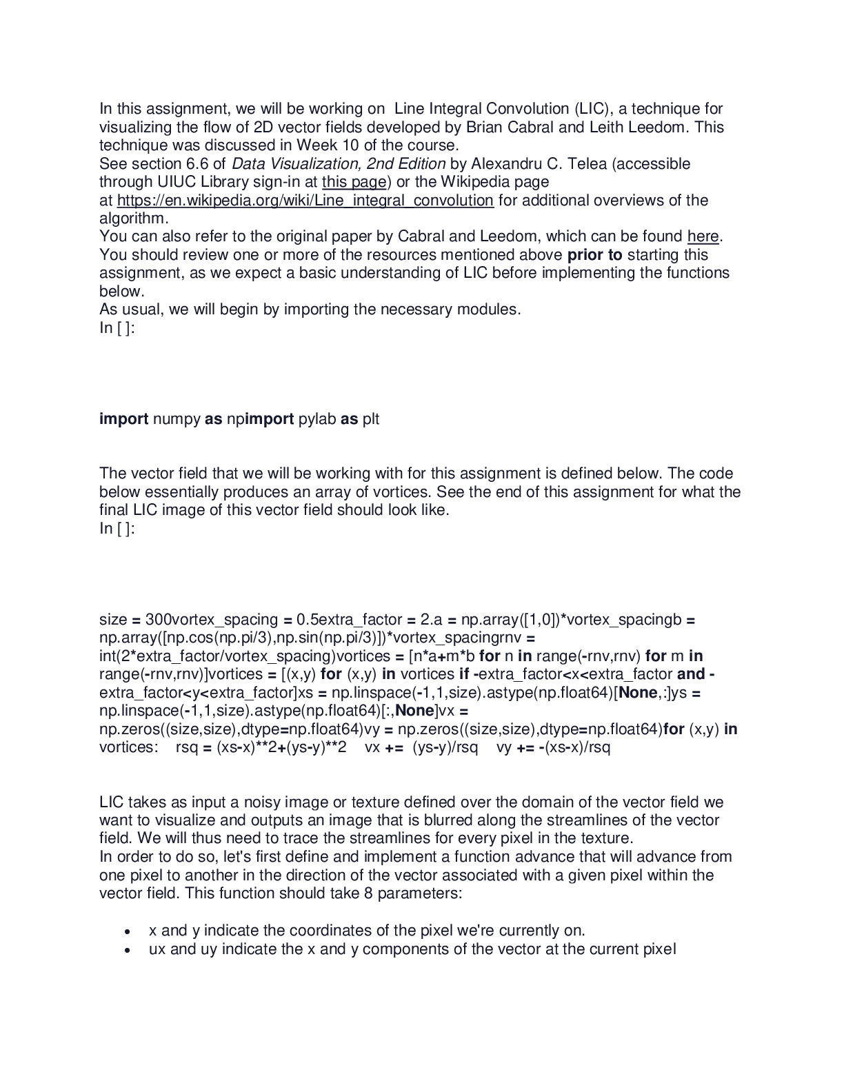
University of Illinois, Urbana Champaign CS CS 519 Scientific VIsualization. In this assignment, we will be working on Line Integral Convolution (LIC), a technique for visualizing the flow of 2D vector fields developed by Brian Cabral and Leith Leedom.

Document Content and Description Below

University of Illinois, Urbana Champaign CS CS 519 In this assignment, we will be working on Line Integral Convolution (LIC), a technique for visualizing the flow of 2D vector fields developed b... y Brian Cabral and Leith Leedom. This technique was discussed in Week 10 of the course. See section 6.6 of Data Visualization, 2nd Edition by Alexandru C. Telea (accessible through UIUC Library sign-in at this page) or the Wikipedia page at https://en.wikipedia.org/wiki/Line_integral_convolution for additional overviews of the algorithm. You can also refer to the original paper by Cabral and Leedom, which can be found here. You should review one or more of the resources mentioned above prior to starting this assignment, as we expect a basic understanding of LIC before implementing the functions below. As usual, we will begin by importing the necessary modules. In [ ]: import numpy as npimport pylab as plt The vector field that we will be working with for this assignment is defined below. The code below essentially produces an array of vortices. See the end of this assignment for what the final LIC image of this vector field should look like. In [ ]: size = 300​vortex_spacing = 0.5extra_factor = 2.​a = np.array([1,0])*vortex_spacingb = np.array([np.cos(np.pi/3),np.sin(np.pi/3)])*vortex_spacingrnv = int(2*extra_factor/vortex_spacing)vortices = [n*a+m*b for n in range(-rnv,rnv) for m in range(-rnv,rnv)]vortices = [(x,y) for (x,y) in vortices if -extra_factor<x<extra_factor and -extra_factor<y<extra_factor]​​xs = np.linspace(-1,1,size).astype(np.float64)[None,:]ys = np.linspace(-1,1,size).astype(np.float64)[:,None]​vx = np.zeros((size,size),dtype=np.float64)vy = np.zeros((size,size),dtype=np.float64)for (x,y) in vortices: rsq = (xs-x)**2+(ys-y)**2 vx += (ys-y)/rsq vy += -(xs-x)/rsq LIC takes as input a noisy image or texture defined over the domain of the vector field we want to visualize and outputs an image that is blurred along the streamlines of the vector field. We will thus need to trace the streamlines for every pixel in the texture. In order to do so, let's first define and implement a function advance that will advance from one pixel to another in the direction of the vector associated with a given pixel within the vector field. This function should take 8 parameters: x and y indicate the coordinates of the pixel we're currently on. ux and uy indicate the x and y components of the vector at the current pixel fx and fy indicate the current subpixel position (treating the current pixel as a unit square where (0,0) represents the top-left of the pixel, while (1,1) represents the bottom-right of the pixel). nx and ny indicate the total number of pixels along the x and y axes within the domain of the entire vector field. advance() should return a 4-tuple consisting of updated x, y, fx, and fy values. These values should be updated by: reading the current pixel / subpixel position given by x, y, fx, and fy calculating tx and ty as the time it takes to reach the next pixel along each axis given fx, fy, ux and uy determining whether the next pixel reached will be on the x-axis or on the y-axis, and whether we are moving forward or backward along that axis using tx, ty, ux, uy, and the results of step (3) to update x, y, fx, and fy in the same order we cross pixel boundaries after min(tx,ty) units of time (i.e., advance far enough to cross a pixel boundary and no farther) Your implementation should also handle the two special cases where advance() would return a pixel outside the vector field, or where ux and uy are both zero vectors. In the first case, x and y should just be clamped to the boundaries of the vector field. In the second case, you could actually interpolate the vector field value at that pixel, but for the purpose of this assignment, you can just return None. Rounding should not be needed or used within your implementation. In [ ]: def advance(ux, uy, x, y, fx, fy, nx, ny): """ Move to the next pixel in the direction of the vector at the current pixel.​ Parameters ---------- ux : float Vector x component. uy :float Vector y component. x : int Pixel x index. y : int Pixel y index. fx : float Position along x in the pixel unit square. fy : float Position along y in the pixel unit square. nx : int Number of pixels along x. ny : int Number of pixels along y. Returns ------- x : int Updated pixel x index. y : int Updated pixel y index. fx : float Updated position along x in the pixel unit square. fy : float Updated position along y in the pixel unit square. """ # YOUR CODE HERE raise NotImplementedError In [ ]: ### Please DO NOT hard-code the answers as we will also be using hidden test cases when grading your submission.x_1, y_1, fx_1, fy_1 = advance(-19.09, 14.25, 0, 0, 0.5, 0.5, 10, 10)​np.testing.assert_allclose(x_1, 0, atol=0.01,rtol=0)np.testing.assert_allclose(y_1, 0, atol=0.01,rtol=0)np.testing.assert_allclose(fx_1, 1, atol=0.01,rtol=0)np.testing.assert_allclose(fy_1, 0.873, atol=0.01,rtol=0)​x_2, y_2, fx_2, fy_2 = advance(14.25, -10.53, 1, 0, 0, 0.13, 10, 10)​np.testing.assert_allclose(x_2, 1, atol=0.01,rtol=0)np.testing.assert_allclose(y_2, 0, atol=0.01,rtol=0)np.testing.assert_allclose(fx_2, 0.176, atol=0.01,rtol=0)np.testing.assert_allclose(fy_2, 1, atol=0.01,rtol=0)​x_3, y_3, fx_3, fy_3 = advance(-10.29, 10.59, 1, 1, 0.67, 0, 10, 10)​np.testing.assert_allclose(x_3, 0, atol=0.01,rtol=0)np.testing.assert_allclose(y_3, 1, atol=0.01,rtol=0)np.testing.assert_allclose(fx_3, 1, atol=0.01,rtol=0)np.testing.assert_allclose(fy_3, 0.690, atol=0.01,rtol=0) Next, let's define and implement the function compute_streamline(), which we will use to trace the streamline centered on a given pixel and apply the convolution kernel to the streamline. We will essentially take an average of the values at all of the pixels along the streamline (using the grey-values from our noisy input texture). These values should also be weighted by the kernel function, where the weight of the kernel function should decrease with distance away from the central pixel. This function takes 6 parameters: vx and vy are 2D arrays containing the x- and y-components respectively of the vector field. px and py indicate the coordinates of the pixel for which we are tracing the streamline. texture indicates the input 2D texture that will be distorted by the vector field kernel is a weighted convolution kernel (i.e., a 1D array symmetric around its middle element, where the middle element is the largest value and all other elements in the array are values decreasing with distance from the middle). The size of kernel is approximately 2L+1 where L is the fixed maximal distance in one direction (i.e. forward or backward) of the streamline. The compute_streamline() function should return the weighted sum of values at each pixel along the streamline centered on (px,py) by doing the following: Initializing the subpixel position (fx,fy) to the center of the pixel (px,py), where fx and fy function as in advance() above Computing a running weighted sum of pixel values along a streamline, using advance to move to each next pixel in the streamline in either direction. Should be able to handle: Center pixel Forward direction (starting from center pixel, increasing to maximal distance L) Backward direction (starting from center pixel, decreasing to -L) (hint: negate the vector passed to advance()) As before, you will need to handle the case of a zero vector (i.e., whenever it returns None) by halting forward / backward iteration along the streamline. You may assume that the shape of vx, vy, and texture are all identical. Also, note that the 2D arrays vx, vy, and texture are stored in memory in (y,x) order, so be sure to index them properly. As before, rounding should not be needed or used within your implementation. For reference, this function is effectively computing the numerator of Equation 6.14 in Section 6.6 of the Data Visualization textbook. A visual reference from the textbook has been included below as well. In [ ]: def compute_streamline(vx, vy, texture, px, py, kernel): """ Return the convolution of the streamline for the given pixel (px, py). Parameters ---------- vx : array (ny, nx) Vector field x component. vy : array (ny, nx) Vector field y component. texture : array (ny,nx) The input texture image that will be distorted by the vector field. px : int Pixel x index. py : int Pixel y index. kernel : 1D array The convolution kernel: an array weighting the texture along the stream line. The kernel should be symmetric. fx : float Position along x in the pixel unit square. fy : float Position along y in the pixel unit square. nx : int Number of pixels along x. ny : int Number of pixels along y. Returns ------- sum : float Weighted sum of values at each pixel along the streamline that starts at center of pixel (px,py) """ # YOUR CODE HERE raise NotImplementedError In [ ]: ### Please DO NOT hard-code the answers as we will also be using hidden test cases when grading your submission.size_test = 100​# Generate 100x100 random noise texturenp.random.seed(123)texture = np.random.rand(size_test, size_test).astype(np.float64)​# Regenerate vector field with new dimensionsxs = np.linspace(-1,1,size_test).astype(np.float64)[None,:]ys = np.linspace(-1,1,size_test).astype(np.float64)[:,None]​vx = np.zeros((size_test,size_test),dtype=np.float64)vy = np.zeros((size_test,size_test),dtype=np.float64)for (x,y) in vortices: rsq = (xs-x)**2+(ys-y)**2 vx += (ys-y)/rsq vy += -(xs-x)/rsq # Generate sinusoidal kernel functionL = 5 #Radius of the kernelkernel = np.sin(np.arange(2*L+1)*np.pi/(2*L+1)).astype(np.float64)​np.testing.assert_allclose(compute_streamline(vx, vy, texture, 9, 9, kernel), 3.622, atol=0.01,rtol=0)np.testing.assert_allclose(compute_streamline(vx, vy, texture, 30, 82, kernel), 5.417, atol=0.01,rtol=0)np.testing.assert_allclose(compute_streamline(vx, vy, texture, 99, 99, kernel), 4.573, atol=0.01,rtol=0) Finally, we will define and implement a function lic() that returns a 2D array corresponding to an image distorted by a vector field using some symmetric convolution kernel. As in the compute_streamline() function above: vx and vy are 2D arrays containing the x- and y-components respectively of some vector field texture indicates the input 2D texture that will be distorted by the vector field kernel is the weighted convolution kernel itself. The lic() function should just iterate over each pixel in texture, computing the streamline at that pixel by using the output of compute_streamline() and normalizing it with respect to the sum of weights within kernel (i.e., computing the denominator of Equation 6.14 referenced above). Once again, rounding should not be needed or used within your implementation. In [ ]: def lic(vx, vy, texture, kernel): """ Return an image of the texture array blurred along the local vector field orientation. Parameters ---------- vx : array (ny, nx) Vector field x component. vy : array (ny, nx) Vector field y component. texture : array (ny,nx) The input texture image that will be distorted by the vector field. kernel : 1D array The convolution kernel: an array weighting the texture along the stream line. The kernel should be symmetric.​ Returns ------- result : array(ny,nx) An image of the texture convoluted along the vector field streamlines.​ """ # YOUR CODE HERE raise NotImplementedError In [ ]: ### Please DO NOT hard-code the answers as we will also be using hidden test cases when grading your submission.size_test = 100​# Generate 100x100 random noise texturenp.random.seed(123)texture = np.random.rand(size_test, size_test).astype(np.float64)​# Regenerate vector field with new dimensionsxs = np.linspace(-1,1,size_test).astype(np.float64)[None,:]ys = np.linspace(-1,1,size_test).astype(np.float64)[:,None]​vx = np.zeros((size_test,size_test),dtype=np.float64)vy = np.zeros((size_test,size_test),dtype=np.float64)for (x,y) in vortices: rsq = (xs-x)**2+(ys-y)**2 vx += (ys-y)/rsq vy += -(xs-x)/rsq # Generate sinusoidal kernel functionL = 5 #Radius of the kernelkernel = np.sin(np.arange(2*L+1)*np.pi/(2*L+1)).astype(np.float64) ​result = lic(vx, vy, texture, kernel)​np.testing.assert_allclose(result[50][50], 0.566, atol=0.01,rtol=0)np.testing.assert_allclose(result[99][99], 0.657, atol=0.01,rtol=0)np.testing.assert_allclose(result[28][36], 0.405, atol=0.01,rtol=0) We are now ready to test our line integral convolution! Below, we create a 300x300 array of random pixel noise. In [ ]: size = 300​np.random.seed(123)texture = np.random.rand(size, size).astype(np.float64)plt.imshow(texture, cmap="gray") Now let's regenerate our vector field (defined at the top of the notebook) to match the dimensions of our texture. In [ ]: xs = np.linspace(-1,1,size).astype(np.float64)[None,:]ys = np.linspace(-1,1,size).astype(np.float64)[:,None]​vx = np.zeros((size,size),dtype=np.float64)vy = np.zeros((size,size),dtype=np.float64)for (x,y) in vortices: rsq = (xs-x)**2+(ys-y)**2 vx += (ys-y)/rsq vy += -(xs-x)/rsq We will use the same sinusoidal kernel as with the tests for each function, but this time we will set the maximal distance L to be 10. This means the size of the kernel will be 2*L+1 = 21. In [ ]: L = 10 # Radius of the kernelkernel = np.sin(np.arange(2*L+1)*np.pi/(2*L+1)).astype(np.float64) Finally, we will generate a new image using our kernel function, vector field, and random noise texture as all defined above. Please note that depending on how you implemented the functions above, generating this image may take anywhere between 5 and 60 seconds. In [ ]: image = lic(vx, vy, texture, kernel) In [ ]: plt.imshow(image, cmap='viridis') If your implementation is correct, you should see an image very similar to the one below. . This basic implementation of LIC does not consider the magnitude of the vectors or their sign. You can further experiment with this implementation by using magnitude to color the image, for example. The end of the lecture video on LIC provides a brief explanation for how you can do so. [Show More]

Last updated: 1 year ago

Preview 1 out of 11 pages