Statistics > QUESTIONS & ANSWERS > Harvard University - STATS 139: Introduction to Data Analysis. Chapter 1-5 (All)
Harvard University - STATS 139: Introduction to Data Analysis. Chapter 1-5
Document Content and Description Below
CHAPTER 1: Introduction to Data Analysis and Decision Making MULTIPLE CHOICE 1. The decision-making concepts covered in Data Analysis & Decision Making book include which of the following? a... . Optimization techniques c. Structured sensitivity analysis b. Decision analysis with uncertainty d. All of these options PTS: 1 MSC: AACSB: Analytic 2. Which of the following statements is not true? a. Dealing with uncertainty includes measuring uncertainty b. Dealing with uncertainty includes modeling uncertainty explicitly into the analysis. c. Dealing with uncertainty includes eliminating uncertainty by using the normal probability distribution d. Uncertainty is a key aspect of most business problems, and dealing with uncertainty requires a basic understanding of probability PTS: 1 MSC: AACSB: Analytic 3. Which of the following is not one of the important themes of your Data Analysis & Decision Making book? a. Data analysis c. Decision making b. Dealing with uncertainty d. Data mining PTS: 1 MSC: AACSB: Analytic 4. Data analysis includes a. data description c. the search for relationships in data b. data inference d. All of these options PTS: 1 MSC: AACSB: Analytic 5. Which of the following is not one of the steps in the modeling process? a. Select scale for model b. Collect and summarize data c. Verify the model d. Present the results e. Implement the model and update it through time PTS: 1 MSC: AACSB: Analytic 6. Which of the following would not be included under data analysis? a. Measuring uncertainty c. Data inference b. Data description d. Search for relationships PTS: 1 MSC: AACSB: Analytic 7. The decision making process includes a. optimization techniques for problems with no uncertainty b. decision analysis for problems with uncertainty c. sensitivity analysis d. All of the above PTS: 1 MSC: AACSB: Analytic 8. Which of the following is not one of the types of models described in Data Analysis & Decision Making book? a. Algebraic model c. Scale model b. Spreadsheet model d. Graphical model PTS: 1 MSC: AACSB: Analytic 9. The modeling process discussed in Data Analysis & Decision Making book is a a. seven-step process b. six-step process c. five-step process d. four-step process e. three-step process PTS: 1 MSC: AACSB: Analytic 10. Which of the following is Excel add-in for performing what-if analyses? a. PrecisionTree b. TopRank c. Solver d. @Risk e. StatTools PTS: 1 MSC: AACSB: Analytic 11. Which of the following statements are false? a. The modeling process discussed in Data Analysis & Decision Making book is five- step process b. Dealing with uncertainty requires a basic understanding of probability c. Uncertainty is a key aspect of most business problems d. Data description and data inference are included under data analysis PTS: 1 MSC: AACSB: Analytic 12. Which of the following statements are false? a. Decision-making includes optimization techniques for problems with certainty, decision analysis for problems with certainty, and structured sensitivity analysis. b. Graphical models can be very helpful for simple problems. For complex problems, however, graphical models usually fail to show the important elements of a problem and how they are related. c. Dealing with uncertainty includes measuring uncertainty and modeling uncertainty explicitly into the analysis. d. All of these options PTS: 1 MSC: AACSB: Analytic 13. Which of the following statements are true: a. A fairly recent alternative to algebraic modeling is spreadsheet modeling. Instead of relating various quantities with algebraic equations and inequalities, we relate them in a spreadsheet with cell formulas. b. Data are usually meaningless until they are analyzed for trends, patterns, relationships, and other useful information c. Algebraic models, by means of algebraic equations and inequalities, specify a set of relationships in a very precise way. Their main drawback is that they require an ability to work with abstract mathematical symbols. d. When we make inferences from data and search for relationships in data, or when we use decision trees to help make decisions, we must deal with uncertainty. e. All of these options PTS: 1 MSC: AACSB: Analytic 14. Which of the following statements are true? a. Three important themes run through the book. Two of them are in the title: data analysis and decision making. The third is dealing with uncertainty. b. Data analysis includes data description, data inference, and the search for relationships in data c. Decision making includes optimization techniques for problems with no uncertainty, decision analysis for problems with uncertainty, and structured sensitivity analysis. d. Dealing with uncertainty includes measuring uncertainty and modeling uncertainty explicitly into the analysis. e. All of these options PTS: 1 MSC: AACSB: Analytic 15. Which of the following is an Excel add-in for simulation? a. PrecisionTree b. TopRank c. Solver d. @Risk e. StatTools PTS: 1 MSC: AACSB: Analytic TRUE/FALSE 1. Data analysis includes data description, data inference, and the search for relationships in data. ANS: T PTS: 1 MSC: AACSB: Analytic 2. Decision-making includes optimization techniques for problems with certainty, decision analysis for problems with certainty, and structured sensitivity analysis. ANS: F PTS: 1 MSC: AACSB: Analytic 3. Dealing with uncertainty includes measuring uncertainty and modeling uncertainty explicitly into the analysis. ANS: F PTS: 1 MSC: AACSB: Analytic 4. The authors of Data Analysis & Decision Making book described three types of models: graphical models, algebraic models, and spreadsheet models. ANS: T PTS: 1 MSC: AACSB: Analytic 5. Graphical models are the least intuitive type of model. Its purpose is simply to provide enough quantitative details to enable us solve the problem of interest. ANS: F PTS: 1 MSC: AACSB: Analytic 6. Three important themes run through this book: data analysis, decision-making, and dealing with uncertainty. ANS: T PTS: 1 MSC: AACSB: Analytic 7. Graphical models can be very helpful for simple problems. For complex problems, however, graphical models usually fail to show the important elements of a problem and how they are related. ANS: F PTS: 1 MSC: AACSB: Analytic 8. The overall modeling process typically done in the business world always require seven steps: define the problem, collect and summarize data, formulate a model, verify the model, select one or more suitable decisions, present the results to the organization, and finally implement the model and update it through time. ANS: F PTS: 1 MSC: AACSB: Analytic 9. Algebraic models, by means of algebraic equations and inequalities, specify a set of relationships in a very precise way. Their main drawback is that they require an ability to work with abstract mathematical symbols. ANS: T PTS: 1 MSC: AACSB: Analytic 10. Data are usually meaningless until they are analyzed for trends, patterns, relationships, and other useful information. ANS: T PTS: 1 MSC: AACSB: Analytic 11. A fairly recent alternative to algebraic modeling is spreadsheet modeling. Instead of relating various quantities with algebraic equations and inequalities, we relate them in a spreadsheet with cell formulas. ANS: T PTS: 1 MSC: AACSB: Analytic 12. When we use simulation models to help make decisions, we do not deal with uncertainty at all, since we often must make inferences from the simulated data. ANS: F PTS: 1 MSC: AACSB: Analytic 13. When we make inferences from data and search for relationships in data, or when we use decision trees to help make decisions, we must deal with uncertainty. ANS: T PTS: 1 MSC: AACSB: Analytic 14. The @Risk is Excel add-in that can be used to run replications of a simulation, keep track of outputs, create useful charts, and perform sensitivity analyses. ANS: T PTS: 1 MSC: AACSB: Analytic 15. Graphical models are probably the least intuitive and most quantitative type of model. ANS: F PTS: 1 MSC: AACSB: Analytic CHAPTER 2: Describing the Distribution of a Single Variable MULTIPLE CHOICE 1. A sample of a population taken at one particular point in time is categorized as: a. categorical b. discrete c. d. cross-sectional time-series ANS: C PTS: 1 MSC: AACSB: Analytic | AACSB: Statistical Inference 2. If data is stored in a database package, which of the following terms are typically used? a. Fields and records c. Variables and samples b. Cases and columns d. Variables and observations PTS: 1 MSC: AACSB: Analytic 3. Researchers may gain insight into the characteristics of a population by examining a a. mathematical model describing the population b. sample of the population c. description of the population d. replica PTS: 1 MSC: AACSB: Analytic | AACSB: Statistical Inference 4. Numerical variables can be subdivided into which two types? a. Diverse and categorical c. Nominal and progressive b. Discrete and continuous d. Cross-sectional and discrete PTS: 1 MSC: AACSB: Analytic 5. Gender and State are examples of which type of data? a. Discrete data c. Categorical data b. Continuous data d. Ordinal data PTS: 1 MSC: AACSB: Analytic | AACSB: Descriptive Statistics 6. Which of the following indicates how many observations fall into various categories? a. The Likert scale c. The sample table b. The frequency table d. The tabulation scale PTS: 1 MSC: AACSB: Analytic | AACSB: Descriptive Statistics 7. Data that arise from counts are called: a. continuous data c. counted data b. nominal data d. discrete data PTS: 1 MSC: AACSB: Analytic 8. A histogram that is positively skewed is also called a. skewed to the right c. balanced b. skewed to the left d. symmetric PTS: 1 MSC: AACSB: Analytic 9. A histogram that has exactly two peaks is called a a. unimodal distribution c. skewed distribution b. bimodal distribution d. scatterplot PTS: 1 MSC: AACSB: Analytic 10. A histogram that has a single peak and looks approximately the same to the left and right of the peak is called: a. bimodal b. symmetric c. d. balanced proportional ANS: B PTS: 1 MSC: AACSB: Analytic 11. A variable is classified as ordinal if: a. there is a natural ordering of categories b. there is no natural ordering of categories c. the data arise from continuous measurements d. we track the variable through a period of time PTS: 1 MSC: AACSB: Analytic 12. In order for the characteristics of a sample to be generalized to the entire population, it should be: a. symbolic of the population c. representative of the population b. typical of the population d. illustrative of the population PTS: 1 MSC: AACSB: Analytic | AACSB: Statistical Inference 13. When we look at a time series plot, we usually look for which two things? a. “Is there an observable trend?” and “Is there a seasonal pattern?” b. “Is there an observable trend” and “Can we make predictions?” c. “Is the sample representative?” and “Is there a seasonal pattern?” d. “Is there an observable trend?” and “Is the trend symmetric?” PTS: 1 MSC: AACSB: Analytic 14. Which of the following are possible categorizations of data type? a. Numerical versus categorical (with subcategories nominal, ordinal) b. Discrete versus continuous c. Cross-sectional versus time series d. All of these options e. Two of these options PTS: 1 MSC: AACSB: Analytic 15. Which of the following are the two most commonly used measures of variability? a. Variance and median b. Variance and standard deviation c. Mean and variance d. Mean and range e. First quartile and third quartile PTS: 1 MSC: AACSB: Analytic | AACSB: Descriptive Statistics 16. The median can also be described as: a. the middle observation when the data values are arranged in ascending order b. the second quartile c. the 50th percentile d. All of these options PTS: 1 MSC: AACSB: Analytic | AACSB: Descriptive Statistics 17. The difference between the first and third quartile is called the a. interquartile range b. interdependent range c. unimodal range d. bimodal range e. mid range PTS: 1 MSC: AACSB: Analytic | AACSB: Descriptive Statistics 18. If a value represents the 95th percentile, this means that a. 95% of all values are below this value b. 95% of all values are above this value c. 95% of the time you will observe this value d. there is a 5% chance that this value is incorrect e. there is a 95% chance that this value is correct PTS: 1 MSC: AACSB: Analytic | AACSB: Descriptive Statistics 19. For a boxplot, the point inside the box indicates the location of the a. mean b. median c. d. minimum value maximum value ANS: A PTS: 1 MSC: AACSB: Analytic | AACSB: Descriptive Statistics 20. For a boxplot, the vertical line inside the box indicates the location of the a. mean b. median c. mode d. minimum value e. maximum value PTS: 1 MSC: AACSB: Analytic | AACSB: Descriptive Statistics 21. Which of the following are the three most common measures of central location? a. Mean, median, and mode b. Mean, variance, and standard deviation c. Mean, median, and variance d. Mean, median, and standard deviation e. First quartile, second quartile, and third quartile PTS: 1 MSC: AACSB: Analytic | AACSB: Descriptive Statistics 22. The length of the box in the boxplot portrays the a. mean b. median c. range d. interquartile range e. third quartile PTS: 1 MSC: AACSB: Analytic | AACSB: Descriptive Statistics 23. Suppose that a histogram of a data set is approximately symmetric and "bell shaped". Approximately what percent of the observations are within two standard deviations of the mean? a. 50% b. 68% c. 95% d. 99.7% e. 100% PTS: 1 MSC: AACSB: Analytic | AACSB: Statistical Inference 24. The mode is best described as the a. middle observation b. same as the average c. 50th percentile d. most frequently occurring value e. third quartile PTS: 1 MSC: AACSB: Analytic | AACSB: Descriptive Statistics 25. For a boxplot, the box itself represents what percent of the observations? a. lower 25% b. middle 50% c. upper 75% d. upper 90% e. 100% PTS: 1 MSC: AACSB: Analytic | AACSB: Descriptive Statistics 26. Which of the following statements is true for the following data values: 7, 5, 6, 4, 7, 8, and 12? a. The mean, median and mode are all equal b. Only the mean and median are equal c. Only the mean and mode are equal d. Only the median and mode are equal PTS: 1 MSC: AACSB: Analytic | AACSB: Descriptive Statistics 27. In a histogram, the percentage of the total area which must be to the left of the median is: a. exactly 50% b. less than 50% if the distribution is skewed to the left c. more than 50% if the distribution is skewed to the right d. between 25% and 50% if the distribution is symmetric and unimodal PTS: 1 MSC: AACSB: Analytic | AACSB: Descriptive Statistics 28. The average score for a class of 30 students was 75. The 20 male students in the class averaged 70. The 10 female students in the class averaged: a. 75 b. 85 c. 60 d. 70 e. 80 PTS: 1 MSC: AACSB: Analytic | AACSB: Descriptive Statistics 29. Which of the following statements is true? a. The sum of the deviations from the mean is always zero b. The sum of the squared deviations from the mean is always zero c. The range is always smaller than the variance d. The standard deviation is always smaller than the variance PTS: 1 MSC: AACSB: Analytic | AACSB: Descriptive Statistics 30. Expressed in percentiles, the interquartile range is the difference between the a. 10th and 60th percentiles b. 15th and 65th percentiles c. 20th and 70th percentiles d. 25th and 75th percentiles e. 35th and 85th percentiles PTS: 1 MSC: AACSB: Analytic | AACSB: Descriptive Statistics 31. A sample of 20 observations has a standard deviation of 4. The sum of the squared deviations from the sample mean is: a. 400 b. 320 c. 304 d. 288 e. 180 PTS: 1 MSC: AACSB: Analytic | AACSB: Descriptive Statistics TRUE/FALSE 1. Age, height, and weight are examples of numerical data. ANS: T PTS: 1 MSC: AACSB: Analytic 2. Data can be categorized as cross-sectional or time series. ANS: T PTS: 1 MSC: AACSB: Analytic 3. All nominal data may be treated as ordinal data. ANS: F PTS: 1 MSC: AACSB: Analytic 4. Four different shapes of histograms are commonly observed: symmetric, positively skewed, negatively skewed, and bimodal. ANS: T PTS: 1 MSC: AACSB: Analytic 5. Categorical variables can be classified as either discrete or continuous. ANS: F PTS: 1 MSC: AACSB: Analytic 6. A skewed histogram is one with a long tail extending either to the right or left. The former is called negatively skewed, and the later is called positively skewed. ANS: F PTS: 1 MSC: AACSB: Analytic CHAPTER 3: Finding Relationships Among Variables MULTIPLE CHOICE 1. To examine relationships between two categorical variables, we can use a. Counts and corresponding charts of the counts b. Scatterplots c. Histograms d. None of these options PTS: 1 MSC: AACSB: Analytic 2. Tables used to display counts of a categorical variable are called a. Crosstabs c. Both of these options b. Contingency tables d. Neither of these options PTS: 1 MSC: AACSB: Analytic 3. The Excel function that allows you to count using more than one criterion is a. COUNTIF b. COUNTIFS c. SUMPRODUCT d. VLOOKUP e. HLOOKUP PTS: 1 MSC: AACSB: Analytic 4. Example of comparison problems include a. Salary broken down by male and female subpopulations b. Cost of living broken down by region of a country c. Recovery rate for a disease broken down by patients who have taken a drug and patients who have taken a placebo d. Starting salary of recent graduates broken down by academic major e. All of these options PTS: 1 MSC: AACSB: Analytic 5. The most common data format is a. Long c. Stacked b. Short d. Unstacked PTS: 1 MSC: AACSB: Analytic 6. A useful way of comparing the distribution of a numerical variable across categories of some categorical variable is a. Side-by-side boxplots c. Both of these options b. Side-by-side histograms d. Neither of these options PTS: 1 MSC: AACSB: Analytic 7. We study relationships among numerical variables using a. Correlation b. Covariance c. Scatterplots d. All of these options e. None of these options PTS: 1 MSC: AACSB: Analytic 8. Scatterplots are also referred to as a. Crosstabs b. Contingency charts c. X-Y charts d. All of these options e. None of these options PTS: 1 MSC: AACSB: Analytic 9. Correlation and covariance measure a. The strength of a linear relationship between two numerical variables b. The direction of a linear relationship between two numerical variables c. The strength and direction of a linear relationship between two numerical variables d. The strength and direction of a linear relationship between two categorical variables e. None of these options PTS: 1 MSC: AACSB: Analytic | AACSB: Descriptive Statistics 10. We can infer that there is a strong relationship between two numerical variables when a. The points on a scatterplot cluster tightly around an upward sloping straight line b. The points on a scatterplot cluster tightly around a downward sloping straight line c. Either of these options d. Neither of these options PTS: 1 MSC: AACSB: Analytic | AACSB: Statistical Inference 11. The limitation of covariance as a descriptive measure of association is that it a. Only captures positive relationships b. Does not capture the units of the variables c. Is very sensitive to the units of the variables d. Is invalid if one of the variables is categorical e. None of these options PTS: 1 MSC: AACSB: Analytic | AACSB: Descriptive Statistics 12. A the correlation is close to 0, then we expect to see a. An upward sloping cluster of points on the scatterplot b. A downward sloping cluster of points c. A cluster of points around a trendline d. A cluster of points with no apparent relationship e. We cannot say what the scatterplot should look like based on the correlation PTS: 1 MSC: AACSB: Analytic | AACSB: Descriptive Statistics 13. We are usually on the lookout for large correlations near a. +1 b. -1 c. d. Either of these options Neither of these options ANS: C PTS: 1 MSC: AACSB: Analytic | AACSB: Descriptive Statistics 14. The correlation is best interpreted a. By itself b. Along with the covariance c. Along with the corresponding scatterplot d. Along with the corresponding contingency chart e. Along with the mean and standard deviation PTS: 1 MSC: AACSB: Analytic | AACSB: Statistical Inference 15. Which of the following are considered measures of association? a. Mean and variance b. Variance and correlation c. Correlation and covariance d. Covariance and variance e. First quartile and third quartile PTS: 1 MSC: AACSB: Analytic | AACSB: Descriptive Statistics 16. Generally speaking, if two variables are unrelated (as one increases, the other shows no pattern), the covariance will be a. a large positive number b. a large negative number c. a positive or negative number close to zero d. a positive or negative number close to +1 or -1 PTS: 1 MSC: AACSB: Analytic | AACSB: Descriptive Statistics 17. A perfect straight line sloping downward would produce a correlation coefficient equal to a. +1 b. –1 c. 0 d. +2 e. –2 PTS: 1 MSC: AACSB: Analytic | AACSB: Descriptive Statistics 18. If Cov(X,Y) = - 16.0, variance of X = 25, variance of Y = 16 then the sample coefficient of correlation r is a. + 1.60 b. – 1.60 c. – 0.80 d. + 0.80 e. Cannot be determined from the given information PTS: 1 MSC: AACSB: Analytic | AACSB: Descriptive Statistics 19. A scatterplot allows one to see: a. whether there is any relationship between two variables b. what type of relationship there is between two variables c. Both options are correct d. Neither option is correct PTS: 1 MSC: AACSB: Analytic | AACSB: Statistical Inference 20. The tool that provides useful information about a data set by breaking it down into subpopulations is the: a. histogram c. pivot table 21. 22. Which of the following statements are false? a. Contingency tables are traditional statistical terms for pivot tables that list counts. b. Time series plot is a chart showing behavior over time of a time series variable. c. Pivot table is a table in Excel that summarizes data broken down by one or more numerical variables. d. None of these options PTS: 1 MSC: AACSB: Analytic 23. Which of the following are true statements of pivot tables? a. They allow us to “slice and dice” data in a variety of ways. b. Statisticians often refer to them as contingency tables or crosstabs. c. Pivot tables can list counts, averages, sums, and other summary measures, whereas contingency tables list only counts. d. All of these options PTS: 1 MSC: AACSB: Analytic TRUE/FALSE 1. Counts for categorical variable are often expressed as percentages of the total. ANS: T PTS: 1 MSC: AACSB: Analytic 2. An example of a joint category of two variables is the count of all non-drinkers who are also nonsmokers. ANS: T PTS: 1 MSC: AACSB: Analytic 3. Joint categories for categorical variables cannot be used to make inferences about the relationship between the individual categorical variables. ANS: F PTS: 1 MSC: AACSB: Analytic 4. Problems in data analysis where we want to compare a numerical variable across two or more subpopulations are called comparison problems. ANS: T PTS: 1 MSC: AACSB: Analytic 5. Side-by-side boxplots allow you to quickly see how two or more categories of a numerical variable compare ANS: T PTS: 1 MSC: AACSB: Analytic 6. We must specify appropriate bins for side-by-side histograms in order to make fair comparisons of distributions by category. ANS: T PTS: 1 MSC: AACSB: Analytic 7. Correlation and covariance can be used to examine relationships between numerical variables and categorical variables that have been coded numerically. ANS: F PTS: 1 MSC: AACSB: Analytic | AACSB: Descriptive Statistics 8. A trend line on a scatterplot is a line or a curve that fits the scatter as well as possible ANS: T PTS: 1 MSC: AACSB: Analytic 9. To form a scatterplot of X versus Y, X and Y must be paired ANS: T PTS: 1 MSC: AACSB: Analytic 10. Correlation has the advantage of being in the same original units as the X and Y variables ANS: F PTS: 1 MSC: AACSB: Analytic | AACSB: Descriptive Statistics 11. Correlation is a single-number summary of a scatterplot ANS: T PTS: 1 MSC: AACSB: Analytic | AACSB: Descriptive Statistics 12. We do not even try to interpret correlations numerically except possibly to check whether they are positive or negative ANS: F PTS: 1 MSC: AACSB: Analytic | AACSB: Statistical Inference 13. The cutoff for defining a large correlation is >0.7 or <-0.7. ANS: F PTS: 1 MSC: AACSB: Analytic | AACSB: Descriptive Statistics 14. Generally speaking, if two variables are unrelated, the covariance will be a positive or negative number close to zero ANS: T PTS: 1 MSC: AACSB: Analytic | AACSB: Statistical Inference 15. The correlation between two variables is a unitless and is always between –1 and +1. ANS: T PTS: 1 MSC: AACSB: Analytic | AACSB: Descriptive Statistics 16. If the standard deviations of X and Y are 15.5 and 10.8, respectively, and the covariance of X and Y is 128.8, then the coefficient of correlation r is approximately 0.77. ANS: T PTS: 1 MSC: AACSB: Analytic | AACSB: Descriptive Statistics 17. It is possible that the data points are close to a curve and have a correlation close to 0, because correlation is relevant only for measuring linear relationships. ANS: T PTS: 1 MSC: AACSB: Analytic | AACSB: Descriptive Statistics 18. If the coefficient of correlation r = 0 .80, the standard deviations of X and Y are 20 and 25, respectively, then Cov(X, Y) must be 400. ANS: T PTS: 1 MSC: AACSB: Analytic | AACSB: Descriptive Statistics 19. The advantage that the coefficient of correlation has over the covariance is that the former has a set lower and upper limit. ANS: T PTS: 1 MSC: AACSB: Analytic | AACSB: Descriptive Statistics 20. If the standard deviation of X is 15, the covariance of X and Y is 94.5, the coefficient of correlation r = 0.90, then the variance of Y is 7.0. ANS: F PTS: 1 MSC: AACSB: Analytic | AACSB: Descriptive Statistics 21. The scatterplot is a graphical technique used to describe the relationship between two numerical variables. ANS: T PTS: 1 MSC: AACSB: Analytic | AACSB: Descriptive Statistics 22. Statisticians often refer to the pivot tables as contingency tables or crosstabs. ANS: T PTS: 1 MSC: AACSB: Analytic | AACSB: Descriptive Statistics 23. If we draw a straight line through the points in a scatterplot and most of the points fall close to the line, there is a strong positive linear relationship between the two variables. ANS: F PTS: 1 MSC: AACSB: Analytic | AACSB: Descriptive Statistics SHORT ANSWER NARRBEGIN: SA_47_49 Below you will find current annual salary data and related information for 30 employees at Gamma Technologies, Inc. These data include each selected employees gender (1 for female; 0 for male), age, number of years of relevant work experience prior to employment at Gamma, number of years of employment at Gamma, the number of years of post-secondary education, and annual salary. The tables of correlations and covariances are presented below. Table of Correlations Gender Age Prior Exp Gamma Exp Education Salary Gender 1.000 Age -0.111 1.000 Prior Exp 0.054 0.800 1.000 Gamma Exp -0.203 0.916 0.587 1.000 Education -0.039 0.518 0.434 0.342 1.000 Salary -0.154 0.923 0.723 0.870 0.617 1.000 Table of Covariances (variances on the diagonal) Gender Age Prior Exp Gamma Exp Education Salary Gender 0.259 Age -0.633 134.051 Prior Exp 0.117 39.060 19.045 Gamma Exp -0.700 72.047 17.413 49.421 Education -0.033 9.951 3.140 3.987 2.947 Salary -1825.97 249702.35 73699.75 143033.29 24747.68 584640062 NARREND 1. Which two variables have the strongest linear relationship with annual salary? ANS: Age at 0.923 and Gamma experience at 0.870 have the strongest linear relationship with annual salary. PTS: 1 MSC: AACSB: Analytic | AACSB: Statistical Inference 2. For which of the two variables, number of years of prior work experience or number of years of post-secondary education, is the relationship with salary stronger? Justify your answer. ANS: Prior work experience is stronger at 0.723 versus 0.617 for number of years of post-secondary education. PTS: 1 MSC: AACSB: Analytic | AACSB: Statistical Inference 3. How would you characterize the relationship between gender and annual salary? ANS: It is a somewhat weak relationship at –0.154. Also, the negative value tells us that the salaries are decreasing as the gender value increases. This indicates that the salaries are lower for females (1) than for males (0). PTS: 1 MSC: AACSB: Analytic | AACSB: Statistical Inference 4. The percentage of the US population without health insurance coverage for samples from the 50 states and District of Columbia for both 2003 and 2004 produced the following table of correlations. Table of Correlations: Percent 2003 Percent 2004 What does the table for the two given sets of percentages tell you in this case? ANS: There is a very large positive correlation between these two sets of percentages. This indicates that the percentages tend to move together, although not perfectly. PTS: 1 MSC: AACSB: Analytic | AACSB: Statistical Inference NARRBEGIN: SA_51_53 An economic development researcher wants to understand the relationship between the average monthly expenditure on utilities for households in a particular middle-class neighborhood and each of the following household variables: family size, approximate location of the household within the neighborhood, and indication of whether those surveyed owned or rented their home, gross annual income of the first household wage earner, gross annual income of the second household wage earner (if applicable), size of the monthly home mortgage or rent payment, and the total indebtedness (excluding the value of a home mortgage) of the household. The correlation for each pairing of variables are shown in the table below: Table of correlations NARREND 5. Which of the variables have a positive linear relationship with the household’s average monthly expenditure on utilities? ANS: Ownership has a strong positive linear relationship with the average expenditure on utilities. Also, family size, income of the first household wage earner, income of the second household wage earned, monthly home mortgage or rent payment, and the total indebtedness of the household have moderate to weak positive relationships with the average expenditure on utilities. PTS: 1 MSC: AACSB: Analytic | AACSB: Statistical Inference 6. Which of the variables have a negative linear relationship with the household’s average monthly expenditure on utilities? ANS: Location of the household has a weak negative linear relationship with the average expenditure on utilities PTS: 1 MSC: AACSB: Analytic | AACSB: Statistical Inference 7. Which of the variables have essentially no linear relationship with the household’s average monthly expenditure on utilities? ANS: It appears that family size has a very weak relationship with the average expenditure on utilities PTS: 1 MSC: AACSB: Analytic | AACSB: Statistical Inference 8. Three samples, regarding the ages of teachers, are selected randomly as shown below: Sample A: 17 22 20 18 23 Sample B: 30 28 35 40 25 Sample C: 44 39 54 21 52 How is the value of the correlation coefficient r affected in each of the following cases? a) Each X value is multiplied by 4. b) Each X value is switched with the corresponding Y value. c) Each X value is increased by 2. ANS: a) The value of does not change. b) The value of does not change. c) The value of does not change. PTS: 1 MSC: AACSB: Analytic | AACSB: Descriptive Statistics 9. The students at small community college in Iowa apply to study either English or Business. Some administrators at the college are concerned that women are being discriminated against in being allowed admittance, particularly in the business program. Below, you will find two pivot tables that show the percentage of students admitted by gender to the English program and the Business school. The data has also been presented graphically. What do the data and graphs indicate? English program Gender No Yes Total Female 46.0% 54.0% 100% Male 60.8% 39.2% 100% Total 53.5% 46.5% 100% Business school Gender No Yes Total Female 69.2% 30.8% 100% Male 64.1% 35.9% 100% Total 65.4% 34.6% 100% ANS: These data indicate that a smaller percentage of women are being admitted to the business program. Only 30.8% of women are being admitted to the business program compared to 35.9% for men. However, it is also important to note that only 34.6% of all applicants (women and men) are admitted to the business program compared to 46.5% for the English program. Maybe the males should say something about being discriminated against in being admitted to the English program. PTS: 1 MSC: AACSB: Analytic | AACSB: Statistical Inference 10. A sample of 30 schools produced the pivot table shown below for the average percentage of students graduating from high school. Use this table to determine how the type of school (public or Catholic) that students attend affects their chance of graduating from high school. ANS: The percentages in the right column suggest that if we look at all schools, the rate of graduation is much higher in Catholic schools than in public schools. But a look at the breakdowns in the three ethnic group columns shows that this difference is due primarily to schools that are black and Latino. There isn't much difference in graduation rates between Catholic and public schools that are white. PTS: 1 MSC: AACSB: Analytic | AACSB: Statistical Inference 11. A data set from a sample of 399 Michigan families was collected. The characteristics of the data include family size (large or small), number of cars owned by family (1, 2, 3, or 4), and whether family owns a foreign car. Excel produced the pivot table shown below. Use this pivot table to determine how family size and number of cars owned influence the likelihood that a family owns a foreign car. ANS: The pivot table shows that the more cars a family owns, the more likely it is that they own a foreign car (makes sense!). Also, the percentage of large families who own a foreign car is larger than the similar percentage of small families (36.0% versus 10.4%). PTS: 1 MSC: AACSB: Analytic | AACSB: Statistical Inference NARRBEGIN: SA_58_67 A sample of 150 students at a State University was taken after the final business statistics exam to ask them whether they went partying the weekend before the final or spent the weekend studying, and whether they did well or poorly on the final. The following table contains the result. Did Well in Exam Did Poorly in Exam Studying for Exam 60 15 Went Partying 22 53 NARREND 12. Of those in the sample who went partying the weekend before the final exam, what percentage of them did well in the exam? ANS: 22 out of 75, or 29.33% PTS: 1 MSC: AACSB: Analytic | AACSB: Descriptive Statistics 13. Of those in the sample who did well on the final exam, what percentage of them went partying the weekend before the exam? ANS: 22 out of 82, or 26.83% PTS: 1 MSC: AACSB: Analytic | AACSB: Descriptive Statistics 14. What percentage of the students in the sample went partying the weekend before the final exam and did well in the exam? ANS: 22 out of 150, or 14.67% PTS: 1 MSC: AACSB: Analytic | AACSB: Descriptive Statistics 15. What percentage of the students in the sample spent the weekend studying and did well in the final exam? ANS: 60 out of 150, or 40% PTS: 1 MSC: AACSB: Analytic | AACSB: Descriptive Statistics 16. What percentage of the students in the sample went partying the weekend before the final exam and did poorly on the exam? ANS: 53 out of 150, or 35.33% PTS: 1 MSC: AACSB: Analytic | AACSB: Descriptive Statistics 17. If the sample is a good representation of the population, what percentage of the students in the population should we expect to spend the weekend studying and do poorly on the final exam? ANS: 15 out of 150, or 10% PTS: 1 MSC: AACSB: Analytic | AACSB: Descriptive Statistics 18. If the sample is a good representation of the population, what percentage of those who spent the weekend studying should we expect to do poorly on the final exam? ANS: 15 out of 75, or 20% PTS: 1 MSC: AACSB: Analytic | AACSB: Statistical Inference 19. If the sample is a good representation of the population, what percentage of those who did poorly on the final exam should we expect to have spent the weekend studying? ANS: 15 out of 68, or 22.06% PTS: 1 MSC: AACSB: Analytic | AACSB: Statistical Inference 20. Of those in the sample who went partying the weekend before the final exam, what percentage of them did poorly in the exam? ANS: 53 out of 75, or 70.67% PTS: 1 MSC: AACSB: Analytic | AACSB: Descriptive Statistics 21. Of those in the sample who did well in the final exam, what percentage of them spent the weekend before the exam studying? ANS: 60 out of 82, or 73.17% PTS: 1 MSC: AACSB: Analytic | AACSB: Descriptive Statistics 22. A health magazine reported that a man’s weight at birth has a significant impact on the chance that the man will suffer a heart attack during his life. A statistician analyzed a data set for a sample of 798 men, and produced the pivot table and histogram shown below. Determine how birth weight influences the chances that a man will have a heart attack. ANS: The above pivot table shows counts (as percentages of row) of heart attack versus birth weight, where birth weight has been grouped into categories. The percentages in each category with heart attacks have then been plotted versus weight at birth as shown in the histogram. It appears that the likelihood of a heart attack is greatest for light babies, and then decreases steadily, but increases slightly for the heaviest babies. PTS: 1 MSC: AACSB: Analytic 23. The table shown below contains information technology (IT) investment as a percentage of total investment for eight countries during the 1990s. It also contains the average annual percentage change in employment during the 1990s. Explain how these data shed light on the question of whether IT investment creates or costs jobs. (Hint: Use the data to construct a scatterplot) Country % IT % Change Netherlands 2.5% 1.6% Italy 4.1% 2.2% Germany 4.5% 2.0% France 5.5% 1.8% Canada 8.3% 2.7% Japan 8.3% 2.7% Britain 8.3% 3.3% U.S. 12.4% 3.7% ANS: The scatterplot displayed below shows there is a clear and surprisingly consistent upward trend in these data -- the larger the IT investment percentage, the larger the percentage increase in employment (at least among these 8 countries). PTS: 1 MSC: AACSB: Analytic | AACSB: Statistical Inference 24. There are two scatterplots shown below. The first chart shows the relationship between the size of the home and the selling price. The second chart examines the relationship between the number of bedrooms in the home and its selling price. Which of these two variables (the size of the home or the number of bedrooms) seems to have the stronger relationship with the home’s selling price? Justify your answer. ANS: The relationship between selling price and house size (in square feet) seems to be a stronger relationship. The correlation value is higher for house size (0.657 to 0.452). The house size and the number of bedrooms seem to be closely related, but the house size variable seems to offer more information. The number of bedrooms is a discrete variable. PTS: 1 MSC: AACSB: Analytic | AACSB: Statistical Inference 25. The following scatterplot compares the selling price and the appraised value. Is there a linear relationship between these two variables? If so, how would you characterize the relationship? ANS: Yes, there is a linear relationship. Correlation value = 0.877 represents a rather strong relationship. You can also see from the scatterplot, that there is a positive relationship between the selling price and the appraisal value. PTS: 1 MSC: AACSB: Analytic | AACSB: Statistical Inference NARRBEGIN: SA_72_81 A recent survey data collected from 1000 randomly selected Internet users. The characteristics of the users include their gender, age, education, marital status and annual income. Using Excel, the following pivot tables were produced. NARREND 26. Approximate the percentage of these Internet users who are men under the age of 30. ANS: Approximately 19% PTS: 1 MSC: AACSB: Analytic | AACSB: Descriptive Statistics 27. Approximate the percentage of these Internet users who are single with no formal education beyond high school. ANS: Approximately 16% PTS: 1 MSC: AACSB: Analytic | AACSB: Descriptive Statistics 28. Approximate the percentage of these Internet users who are currently employed. ANS: Approximately 77% PTS: 1 MSC: AACSB: Analytic | AACSB: Descriptive Statistics 29. What is the average annual salary of the employed Internet users in this sample? ANS: Approximately $60,564 PTS: 1 MSC: AACSB: Analytic | AACSB: Descriptive Statistics 30. Approximate the percentage of these Internet users who are married with formal education beyond high school. ANS: Approximately 37% PTS: 1 MSC: AACSB: Analytic | AACSB: Descriptive Statistics 31. What percentage of these Internet users who are married. ANS: Approximately 69% PTS: 1 MSC: AACSB: Analytic | AACSB: Descriptive Statistics 32. Approximate the percentage of these Internet users who are in the 58-71 age group. ANS: Approximately 9% PTS: 1 MSC: AACSB: Analytic | AACSB: Descriptive Statistics 33. Approximate the percentage of these internet users who are women. ANS: Approximately 39% PTS: 1 MSC: AACSB: Analytic | AACSB: Descriptive Statistics 34. What percentage of these internet users has formal education beyond high school? ANS: Exactly 52% PTS: 1 MSC: AACSB: Analytic | AACSB: Descriptive Statistics 35. Approximate the percentage of these internet users who are women in the 30-43 age group. ANS: Approximately 15% PTS: 1 MSC: AACSB: Analytic | AACSB: Descriptive Statistics NARRBEGIN: SA_82_84 Economists believe that countries with more income inequality have lower unemployment rates. An economist in 1996 developed the Table below which contains the following information for ten countries during the 1980-1995 time period: • The change from 1980 to 1995 in ratio of the average wage of the top 10% of all wage earners to the median wage • The change from 1980 to 1995 in unemployment rate. Income inequality vs. Unemployment rate Country WIR Change UR Change Germany -6.0% 6.0% France -3.5% 5.6% Italy 1.0% 5.2% Japan 0.0% 0.6% Australia 5.0% 2.4% Sweden 4.0% 5.9% Canada 5.5% 2.0% New Zealand 9.5% 4.0% Britain 15.6% 2.5% U.S. 15.8% -1.8% NARREND 36. Explain why the ratio of the average wage of the top 10% of all wage earners to the median measures income inequality. ANS: If this ratio is high, then a relatively large share of all income is being made by the people in the upper 10% -- hence "inequality". (Of course, by definition, they’re making more than 10% of all income, but this ratio measures how much more.) PTS: 1 MSC: AACSB: Analytic | AACSB: Statistical Inference 37. Do these data help to confirm or contradict the hypothesis that increased wage inequality leads to lower unemployment levels? [Hint: construct a scatterplot] ANS: The scatterplot shown above indicates that except possibly for the one point indicated (Japan), there is a clear downward trend to these points -- when the wage inequality ratio is up (change is positive), the unemployment rate tends to be down (change negative), and vice versa. So these data support the hypothesis. PTS: 1 MSC: AACSB: Analytic | AACSB: Statistical Inference 38. What other data would you need to be more confident that increased income inequality leads to lower unemployment? ANS: The ratio given here is only one measure of income inequality; others might shed more light on the issue. Also, these data are only for 10 countries and for one period of change (1980 to 1995). More data would be useful. PTS: 1 MSC: AACSB: Analytic | AACSB: Statistical Inference 39. A car dealer collected the following information about a sample of 448 Grand Rapids residents: • Exact salaries of these Grand Rapids residents • Education level (completed high school only or completed college) • Income level (low or high) • Car finance (whether or not the last purchased car was financed) Using the education level, income level, and car finance data, he created the three pivot tables shown below. Based on these tables; determine how education and income influence the likelihood that a family finances a car. ANS: The first two pivot tables are slightly different ways of seeing how the percentage that financed varies across the different education, income categories. However, the third pivot table shows how many are in each education/income category. In particular, note that although a high percentage of low income people with a college degree financed their car purchase, there aren't many low income people with a college education. PTS: 1 MSC: AACSB: Analytic | AACSB: Statistical Inference 7. Some histograms have two or more peaks. This is often an indication that the data come from two or more distinct populations. ANS: T PTS: 1 MSC: AACSB: Analytic | AACSB: Statistical Inference 8. A population includes all elements or objects of interest in a study, whereas a sample is a subset of the population used to gain insights into the characteristics of the population. ANS: T PTS: 1 MSC: AACSB: Analytic | AACSB: Statistical Inference 9. A frequency table indicates how many observations fall within each category, and a histogram is its graphical analog. ANS: T PTS: 1 MSC: AACSB: Analytic 10. In the term “frequency table,” frequency refers to the number of data values falling within each category. ANS: T PTS: 1 MSC: AACSB: Analytic 11. Time series data are often graphically depicted on a line chart, which is a plot of the variable of interest over time. ANS: T PTS: 1 MSC: AACSB: Analytic 12. The number of car insurance policy holders is an example of a discrete random variable ANS: T PTS: 1 MSC: AACSB: Analytic 13. A variable (or field) is an attribute, or measurement, on members of a population, whereas an observation (or case or record) is a list of all variable values for a single member of a population. ANS: T PTS: 1 MSC: AACSB: Analytic 14. Phone numbers, Social Security numbers, and zip codes are examples of numerical variables. ANS: F PTS: 1 MSC: AACSB: Analytic 15. Cross-sectional data are data on a population at a distinct point in time, whereas time series data are data collected across time. ANS: T PTS: 1 MSC: AACSB: Analytic 16. Distribution is a general term used to describe the way data are distributed, as indicated by a frequency table or histogram. ANS: T PTS: 1 MSC: AACSB: Analytic 17. Both ordinal and nominal variables are categorical. ANS: T PTS: 1 MSC: AACSB: Analytic 18. A histogram is said to be symmetric if it has a single peak and looks approximately the same to the left and right of the peak. ANS: T PTS: 1 MSC: AACSB: Analytic 19. Suppose that a sample of 10 observations has a standard deviation of 3, then the sum of the squared deviations from the sample mean is 30. ANS: F PTS: 1 MSC: AACSB: Analytic | AACSB: Descriptive Statistics 20. If a histogram has a single peak and looks approximately the same to the left and right of the peak, we should expect no difference in the values of the mean, median, and mode. ANS: T PTS: 1 MSC: AACSB: Analytic | AACSB: Descriptive Statistics 21. The mean is a measure of central location. ANS: T PTS: 1 MSC: AACSB: Analytic | AACSB: Descriptive Statistics 22. The length of the box in the boxplot portrays the interquartile range. ANS: T PTS: 1 MSC: AACSB: Analytic | AACSB: Descriptive Statistics 23. In a positively skewed distribution, the mean is smaller than the median and the median is smaller than the mode. ANS: F PTS: 1 MSC: AACSB: Analytic | AACSB: Descriptive Statistics 24. The value of the standard deviation always exceeds that of the variance. ANS: F PTS: 1 MSC: AACSB: Analytic | AACSB: Descriptive Statistics 25. The difference between the first and third quartiles is called the interquartile range. ANS: T PTS: 1 MSC: AACSB: Analytic | AACSB: Descriptive Statistics 26. The standard deviation is measured in original units, such as dollars and pounds. ANS: T PTS: 1 MSC: AACSB: Analytic | AACSB: Descriptive Statistics 27. The median is one of the most frequently used measures of variability. ANS: F PTS: 1 MSC: AACSB: Analytic | AACSB: Descriptive Statistics 28. Assume that the histogram of a data set is symmetric and bell shaped, with a mean of 75 and standard deviation of 10. Then, approximately 95% of the data values were between 55 and 95. ANS: T PTS: 1 MSC: AACSB: Analytic | AACSB: Descriptive Statistics 29. Abby has been keeping track of what she spends to rent movies. The last seven week's expenditures, in dollars, were 6, 4, 8, 9, 6, 12, and 4. The mean amount Abby spends on renting movies is $7. ANS: T PTS: 1 MSC: AACSB: Analytic | AACSB: Descriptive Statistics 30. Expressed in percentiles, the interquartile range is the difference between the 25th and 75th percentiles. ANS: T PTS: 1 MSC: AACSB: Analytic | AACSB: Descriptive Statistics 31. The value of the mean times the number of observations equals the sum of all of the data values. ANS: T PTS: 1 MSC: AACSB: Analytic | AACSB: Descriptive Statistics 32. The difference between the largest and smallest values in a data set is called the range. ANS: T PTS: 1 MSC: AACSB: Analytic | AACSB: Descriptive Statistics 33. There are four quartiles that divide the values in a data set into four equal parts. ANS: F PTS: 1 MSC: AACSB: Analytic | AACSB: Descriptive Statistics 34. Suppose that a sample of 8 observations has a standard deviation of 2.50, then the sum of the squared deviations from the sample mean is 17.50. ANS: F PTS: 1 MSC: AACSB: Analytic | AACSB: Descriptive Statistics 35. The median of a data set with 30 values would be the average of the 15th and the 16th values when the data values are arranged in ascending order. ANS: T PTS: 1 MSC: AACSB: Analytic | AACSB: Descriptive Statistics SHORT ANSWER NARRBEGIN: SA_71_73 A manager for Marko Manufacturing, Inc. has recently been hearing some complaints that women are being paid less than men for the same type of work in one of their manufacturing plants. The boxplots shown below represent the annual salaries for all salaried workers in that facility (40 men and 34 women). NARREND 1. Would you conclude that there is a difference between the salaries of women and men in this plant? Justify your answer. ANS: Yes. The men seem to have higher salaries than the women do in many cases. We can see from the boxplots that the mean and median values for the men are both higher than for the women. You can also see from the boxplots that the middle 50% of salaries for men is above the median for women. This means that if you were in the 25th percentile for men, you would be above the 50th percentile for women. You can also see that the mean and median salaries for the men are about $10,000 above those for the women. PTS: 1 MSC: AACSB: Analytic | AACSB: Statistical Inference 2. How large must a person’s salary should be to qualify as an outlier on the high side? How many outliers are there in these data? ANS: A person’s salary should be somewhere above $70,000. There is one male salary that would be considered an outlier (at approximately $80,000) PTS: 1 MSC: AACSB: Analytic | AACSB: Statistical Inference 3. What can you say about the shape of the distributions given the boxplots above? ANS: They both appear to be slightly skewed to the right (both have a mean > median). The total variation seems to be close for both distributions (with one outlier for the male salaries), but there seems to be more variation in the middle 50% for the women than for the men. There seem to be more men’s salaries clustered more closely around the mean than for the women. PTS: 1 MSC: AACSB: Analytic | AACSB: Statistical Inference NARRBEGIN: SA_74_75 Statistics professor has just given a final examination in his statistical inference course. He is particularly interested in learning how his class of 40 students performed on this exam. The scores are shown below. 77 81 74 77 79 73 80 85 86 73 83 84 81 73 75 91 76 77 95 76 90 85 92 84 81 64 75 90 78 78 82 78 86 86 82 70 76 78 72 93 NARREND 4. What are the mean and median scores on this exam? ANS: Mean = 80.40, Median = 79.50 PTS: 1 MSC: AACSB: Analytic | AACSB: Descriptive Statistics 5. Explain why the mean and median are different. ANS: There are few higher exam scores that tend to pull the mean away from the middle of the distribution. While there is a slight amount of positive skewness in the distribution (skewness = 0.182), the mean and the median are essentially equivalent in this case. PTS: 1 MSC: AACSB: Analytic | AACSB: Descriptive Statistics NARRBEGIN: SA_76_78 The data shown below contains family incomes (in thousands of dollars) for a set of 50 families; sampled in 1980 and 1990. Assume that these families are good representatives of the entire United States. 1980 1990 1980 1990 1980 1990 58 54 33 29 73 69 6 2 14 10 26 22 59 55 48 44 64 70 71 57 20 16 59 55 30 26 24 20 11 7 38 34 82 78 70 66 36 32 95 97 31 27 33 29 12 8 92 88 72 68 93 89 115 111 100 96 100 102 62 58 1 0 51 47 23 19 27 23 22 18 34 30 22 47 50 75 36 61 141 166 124 149 125 150 72 97 113 138 121 146 165 190 118 143 88 113 79 104 96 121 NARREND 6. Find the mean, median, standard deviation, first and third quartiles, and the 95th percentile for family incomes in both years. ANS: Mean Median Standard deviation First quartile Third quartile 95th percentile Income 1980 Income 1990 62.820 67.120 59.000 57.500 39.786 48.087 30.250 27.500 92.750 97.000 124.550 149.55 PTS: 1 MSC: AACSB: Analytic | AACSB: Descriptive Statistics 7. The Republicans claim that the country was better off in 1990 than in 1980, because the average income increased. Do you agree? ANS: It is true that the mean increased slightly, but the median decreased and the standard deviation increased. The 95th percentile shows that the mean increase might be because the rich got richer. PTS: 1 MSC: AACSB: Analytic | AACSB: Statistical Inference 8. Generate a boxplot to summarize the data. What does the boxplot indicate? ANS: The boxplot shows that there is not much difference between the two populations. PTS: 1 MSC: AACSB: Analytic | AACSB: Statistical Inference NARRBEGIN: SA_79_81 In an effort to provide more consistent customer service, the manager of a local fast-food restaurant would like to know the dispersion of customer service times about their average value for the facility’s drive-up window. The table below provides summary measures for the customer service times (in minutes) for a sample of 50 customers collected over the past week. Count 50.000 Mean 0.873 Median 0.885 Standard deviation 0.432 Minimum 0.077 Maximum 1.608 Variance 0.187 Skewness -0.003 NARREND 9. Interpret the variance and standard deviation of this sample. ANS: The variance = 0.187 (minutes squared) and this represents the average of the squared deviations from the mean. The standard deviation = 0.432 (minutes) and is the square root of the variance. Both the variance and standard deviation measure the variation around the mean of the data. However, it is easier to interpret the standard deviation because it is expressed in the same units (minutes) as the values of the random variable (customer service time). PTS: 1 MSC: AACSB: Analytic | AACSB: Statistical Inference 10. Are the empirical rule applicable in this case? If so, apply it and interpret your results. If not, explain why the empirical rule is not applicable here. ANS: Considering that this distribution is only very slightly skewed to the left, it is acceptable to apply the empirical rule as follows: Approximately 68% of the customer service times will fall between 0.873 ± 0.432, that is between 0.441 and 1.305 minutes. Approximately 95% of the customer service times will fall between 0.873 ± 2(0.432), that is between 0.009 and 1.737 minutes. Approximately 99.7% of the customer service times will fall between 0.873 ± 3(0.432), that is between 0 and 2.169 (we set the lower end to zero since service times cannot assume negative values). PTS: 1 MSC: AACSB: Analytic | AACSB: Statistical Inference 11. Explain what would cause the mean to be slightly lower than the median in this case. ANS: The data is slightly skewed to the left. This is causing the mean to be slightly lower than the median. It is important to understand that service times are bounded on the lower end by zero (or it is impossible for the service time to be negative). However, there is no bound on the maximum service time. Therefore, the smaller service times are causing the mean to be somewhat lower than the median. PTS: 1 MSC: AACSB: Analytic | AACSB: Statistical Inference NARRBEGIN: SA_82_85 Below you will find summary measures on salaries for classroom teachers across the United States. You will also find a list of selected states and their average teacher salary. All values are in thousands of dollars. Salaries for classroom teachers across the United States Salary Count 51.000 Mean 35.890 Median 35.000 Standard deviation 6.226 Minimum 26.300 Maximum 50.300 Variance 38.763 First quartile 31.550 Third quartile 40.050 Selected states and their average teacher salary State Salary Alabama 31.3 Colorado 35.4 Connecticut 50.3 Delaware 40.5 Nebraska 31.5 Nevada 36.2 New Hampshire 35.8 New Jersey 47.9 New Mexico 29.6 South Carolina 31.6 South Dakota 26.3 Tennessee 33.1 Texas 32.0 Utah 30.6 Vermont 36.3 Virginia 35.0 Wyoming 31.6 NARREND 12. Which of the states listed paid their teachers average salaries that exceed at least 75% of all average salaries? ANS: Connecticut at 50.3; Delaware at 40.5; and New Jersey at 47.9 (all those > 40.05). PTS: 1 MSC: AACSB: Analytic | AACSB: Statistical Inference 13. Which of the states listed paid their teachers average salaries that are below 75% of all average salaries? ANS: Alabama at 31.3; Nebraska at 31.5; New Mexico at 29.6; South Dakota at 26.3; and Utah at 30.6 (all those < 31.55). PTS: 1 MSC: AACSB: Analytic | AACSB: Statistical Inference 14. What salary amount represents the second quartile? ANS: $35,000 (median) PTS: 1 MSC: AACSB: Analytic | AACSB: Descriptive Statistics 15. How would you describe the salary of Virginia’s teachers compared to those across the entire United States? Justify your answer. ANS: Virginia = $35,000 which is also the median. Virginia is at the 50th percentile or 50% of the teachers’ salaries across the U.S. are below Virginia and 50% of the salaries are above theirs. PTS: 1 MSC: AACSB: Analytic | AACSB: Statistical Inference NARRBEGIN: SA_86_88 Suppose that an analysis of a set of test scores reveals that: , NARREND 16. What do these statistics tell you about the shape of the distribution? ANS: The fact that 40 is greater that 20 indicates that the distribution is skewed to the left. PTS: 1 MSC: AACSB: Analytic | AACSB: Statistical Inference 17. What can you say about the relative position of each of the observations 34, 84, and 104? ANS: Since 34 is less than , the observation 34 is among the lowest 25% of the values. The value 84 is a bit smaller than the middle value, which is 85. Since 105, the value 104 is larger than about 75% of the values. PTS: 1 MSC: AACSB: Analytic | AACSB: Statistical Inference 18. Calculate the interquartile range. What does this tell you about the data? ANS: IQR = 60. This means that the middle 50% of the test scores are between 45 and 105. PTS: 1 MSC: AACSB: Analytic | AACSB: Statistical Inference NARRBEGIN: SA_89_91 The following data represent the number of children in a sample of 10 families from Chicago: 4, 2, 1, 1, 5, 3, 0, 1, 0, and 2. NARREND 19. Compute the mean number of children. ANS: Mean = 1.90 PTS: 1 MSC: AACSB: Analytic | AACSB: Descriptive Statistics 20. Compute the median number of children. ANS: Median = 1.5 PTS: 1 MSC: AACSB: Analytic | AACSB: Descriptive Statistics 21. Is the distribution of the number of children symmetrical or skewed? Why? ANS: The distribution is positively skewed because the mean is larger than the median. PTS: 1 MSC: AACSB: Analytic | AACSB: Descriptive Statistics 22. The data below represents monthly sales for two years of beanbag animals at a local retail store (Month 1 represents January and Month 12 represents December). Given the time series plot below, do you see any obvious patterns in the data? Explain. ANS: This is a representation of seasonal data. There seems to be a small increase in months 3, 4, and 5 and a large increase at the end of the year. The sales of this item seem to peak in December and have a significant drop off in January. PTS: 1 MSC: AACSB: Analytic | AACSB: Statistical Inference 23. An operations management professor is interested in how her students performed on her midterm exam. The histogram shown below represents the distribution of exam scores (where the maximum score is 100) for 50 students. Based on this histogram, how would you characterize the students’ performance on this exam? ANS: Exam scores are fairly normally distributed. Majority of scores (76%) are between 70 and 90 points, while 12% of scores are above 90 and 12% of scores are 70 or below. PTS: 1 MSC: AACSB: Analytic | AACSB: Statistical Inference 24. The proportion of Americans under the age of 18 who are living below the poverty line for each of the years 1959 through 2000 is used to generate the following time series plot. How successful have Americans been recently in their efforts to win “the war against poverty” for the nation’s children? ANS: Americans have been relatively unsuccessful in winning the war on poverty in the 1990s. This is especially true when you compare recent poverty rates with those of the years from 1969 through 1979. However, at least the curve is trending downwards in the most recent years. PTS: 1 MSC: AACSB: Analytic | AACSB: Statistical Inference NARRBEGIN: SA_95_97 A financial analyst collected useful information for 30 employees at Gamma Technologies, Inc. These data include each selected employees gender, age, number of years of relevant work experience prior to employment at Gamma, number of years of employment at Gamma, the number of years of post-secondary education, and annual salary. NARREND 25. Indicate the type of data for each of the six variables included in this set. ANS: Gender – categorical, nominal Age – numerical, continuous Prior experience – numerical, discrete Gamma experience – numerical, discrete Education – numerical, discrete Annual salary – numerical, continuous PTS: 1 MSC: AACSB: Analytic 26. Based on the histogram shown below, how would you describe the age distribution for these data? ANS: The age distribution is skewed slightly to the right. Largest grouping is in the 30-40 range. This means that most workers are above the age of 30 years and only one worker is 20 years old or younger. PTS: 1 MSC: AACSB: Analytic | AACSB: Statistical Inference 27. Based on the histogram shown below, how would you describe the salary distribution for these data? ANS: The salary distribution is skewed to the right. There appears to be several workers who are being paid substantially more than the others. If you eliminate those above $80,000, the salaries are fairly normally distributed around $35,000. PTS: 1 MSC: AACSB: Analytic | AACSB: Statistical Inference NARRBEGIN: SA_98_103 The histogram below represents scores achieved by 250 job applicants on a personality profile. NARREND 28. What percentage of the job applicants scored between 30 and 40? ANS: 10% PTS: 1 MSC: AACSB: Analytic | AACSB: Descriptive Statistics 29. What percentage of the job applicants scored below 60? ANS: 90% PTS: 1 MSC: AACSB: Analytic | AACSB: Descriptive Statistics 30. How many job applicants scored between 10 and 30? ANS: 100 PTS: 1 MSC: AACSB: Analytic | AACSB: Descriptive Statistics 31. How many job applicants scored above 50? ANS: 50 PTS: 1 MSC: AACSB: Analytic | AACSB: Descriptive Statistics 32. Seventy percent of the job applicants scored above what value? ANS: 20 PTS: 1 MSC: AACSB: Analytic | AACSB: Descriptive Statistics 33. Half of the job applicants scored below what value? ANS: 30 PTS: 1 MSC: AACSB: Analytic | AACSB: Descriptive Statistics 34. A question of great interest to economists is how the distribution of family income has changed in the United States during the last 20 years. The summary measures and histograms shown below are generated for a sample of 500 family incomes, using the 1985 and 2005 income for each family in the sample. Summary Measures: Based on these results, discuss as completely as possible how the distribution of family income in the United States changed from 1985 to 2005. ANS: These summary measures say quite a lot. The mean has increased, although the median has decreased. There is also more variation. In fact, the 5th percentile has decreased slightly, whereas the 95th percentile is much larger -- the rich people are getting richer. This behavior is also evident in the two histograms (which use the same categories for ease of comparison). PTS: 1 MSC: AACSB: Analytic | AACSB: Statistical Inference CHAPTER 4: Probability and Probability Distributions MULTIPLE CHOICE 1. Probabilities that cannot be estimated from long-run relative frequencies of events are a. objective probabilities c. complementary probabilities b. subjective probabilities d. joint probabilities PTS: 1 MSC: AACSB: Analytic | AACSB: Probability Concepts 2. The probability of an event and the probability of its complement always sum to: a. 1b. 0 c. d. any value between 0 and 1 any positive value ANS: A PTS: 1 MSC: AACSB: Analytic | AACSB: Probability Concepts 3. If events A and B are mutually exclusive, then the probability of both events occurring simultaneously is equal to a. 0.0 b. 0.5 c. d. 1.0 any value between 0.5 and 1.0 ANS: A PTS: 1 MSC: AACSB: Analytic | AACSB: Probability Concepts 4. Probabilities that can be estimated from long-run relative frequencies of events are a. objective probabilities c. complementary probabilities b. subjective probabilities d. joint probabilities PTS: 1 MSC: AACSB: Analytic | AACSB: Probability Concepts 5. Let A and B be the events of the FDA approving and rejecting a new drug to treat hypertension, respectively. The events A and B are: a. independent c. unilateral b. conditional d. mutually exclusive PTS: 1 MSC: AACSB: Analytic | AACSB: Probability Concepts 6. A function that associates a numerical value with each possible outcome of an uncertain event is called a a. conditional variable c. population variable b. random variable d. sample variable PTS: 1 MSC: AACSB: Analytic | AACSB: Probability Concepts 7. The formal way to revise probabilities based on new information is to use: a. complementary probabilities c. unilateral probabilities b. conditional probabilities d. common sense probabilities PTS: 1 MSC: AACSB: Analytic | AACSB: Probability Concepts 8. is the: a. addition rule c. rule of complements b. commutative rule d. rule of opposites PTS: 1 MSC: AACSB: Analytic | AACSB: Probability Concepts 9. The law of large numbers is relevant to the estimation of a. objective probabilities c. both of these options b. subjective probabilities d. neither of these options PTS: 1 MSC: AACSB: Analytic | AACSB: Probability Concepts 10. A discrete probability distribution: a. lists all of the possible values of the random variable and their corresponding probabilities b. is a tool that can be used to incorporate uncertainty into models c. can be estimated from long-run proportions d. is the distribution of a single random variable PTS: 1 MSC: AACSB: Analytic | AACSB: Probability Concepts 11. Which of the following statements are true? a. Probabilities must be nonnegative b. Probabilities must be less than or equal to 1 c. The sum of all probabilities for a random variable must be equal to 1 d. All of these options are true. PTS: 1 MSC: AACSB: Analytic | AACSB: Probability Concepts 12. If P(A) = P(A|B), then events A and B are said to be a. mutually exclusive c. exhaustive b. independent d. complementary PTS: 1 MSC: AACSB: Analytic | AACSB: Probability Concepts 13. If A and B are mutually exclusive events with P(A) = 0.70, then P(B): a. can be any value between 0 and 1 b. can be any value between 0 and 0.70 c. cannot be larger than 0.30 d. Cannot be determined with the information given PTS: 1 MSC: AACSB: Analytic | AACSB: Probability Concepts 14. If two events are collectively exhaustive, what is the probability that one or the other occurs? a. 0.25 b. 0.50 c. 1.00 d. Cannot be determined from the information given. PTS: 1 MSC: AACSB: Analytic | AACSB: Probability Concepts 15. If two events are collectively exhaustive, what is the probability that both occur at the same time? a. 0.00 b. 0.50 c. 1.00 d. Cannot be determined from the information given. PTS: 1 MSC: AACSB: Analytic | AACSB: Probability Concepts 16. The joint probabilities shown in a table with two rows, and and two columns, and , are as follows: P( and ) = .10, P( and ) = .30, P( and ) = .05, and P( and ) = .55. Then P( | ), calculated up to two decimals, is a. .33 c. .65 b. .35 ANS: D PTS: 1 d. MSC: .67 AACSB: Analytic | AACSB: Probability Concepts 17. If two events are mutually exclusive, what is the probability that one or the other occurs? a. 0.25 b. 0.50 c. 1.00 d. Cannot be determined from the information given. PTS: 1 MSC: AACSB: Analytic | AACSB: Probability Concepts 18. If two events are mutually exclusive, what is the probability that both occur at the same time? a. 0.00 b. 0.50 c. 1.00 d. Cannot be determined from the information given. PTS: 1 MSC: AACSB: Analytic | AACSB: Probability Concepts 19. If two events are mutually exclusive and collectively exhaustive, what is the probability that both occur? a. 0.00 b. 0.50 c. 1.00 d. Cannot be determined from the information given. PTS: 1 MSC: AACSB: Analytic | AACSB: Probability Concepts 20. There are two types of random variables, they are a. discrete and continuous c. complementary and cumulative b. exhaustive and mutually exclusive d. real and unreal PTS: 1 MSC: AACSB: Analytic | AACSB: Probability Concepts 21. If P(A) = 0.25 and P(B) = 0.65, then P(A and B) is: a. 0.25 b. 0.40 c. 0.90 d. Cannot be determined from the information given PTS: 1 MSC: AACSB: Analytic | AACSB: Probability Concepts 22. If two events are independent, what is the probability that they both occur? a. 0 b. 0.50 c. 1.00 d. Cannot be determined from the information given PTS: 1 MSC: AACSB: Analytic | AACSB: Probability Concepts 23. If A and B are any two events with P(A) = .8 and P(B| ) = .7, then P( and B) is a. .56 c. .24 b. .14 d. None of the above PTS: 1 MSC: AACSB: Analytic | AACSB: Probability Concepts 24. Which of the following best describes the concept of marginal probability? a. It is a measure of the likelihood that a particular event will occur, regardless of whether another event occurs. b. It is a measure of the likelihood that a particular event will occur, given that another event has already occurred. c. It is a measure of the likelihood of the simultaneous occurrence of two or more events. d. None of the above. PTS: 1 MSC: AACSB: Analytic | AACSB: Probability Concepts 25. The joint probabilities shown in a table with two rows, and and two columns, and , are as follows: P( and ) = .10, P( and ) = .30, P( and ) = .05, and P( and ) = .55. Then P( | ), calculated up to two decimals, is a. .33 c. .65 b. .35 d. .67 PTS: 1 MSC: AACSB: Analytic | AACSB: Probability Concepts 26. If A and B are mutually exclusive events with P(A) = 0.30 and P(B) = 0.40, then the probability that either A or B or both occur is: 27. TRUE/FALSE 1. If A and B are independent events with P(A) = 0.40 and P(B) = 0.50, then P(A/B) is 0.50. ANS: F PTS: 1 MSC: AACSB: Analytic | AACSB: Probability Concepts 2. A random variable is a function that associates a numerical value with each possible outcome of a random phenomenon. ANS: T PTS: 1 MSC: AACSB: Analytic | AACSB: Probability Concepts 3. Two or more events are said to be exhaustive if one of them must occur. ANS: T PTS: 1 MSC: AACSB: Analytic | AACSB: Probability Concepts 4. You think you have a 90% chance of passing your statistics class. This is an example of subjective probability. ANS: T PTS: 1 MSC: AACSB: Analytic | AACSB: Probability Concepts 5. The number of cars produced by GM during a given quarter is a continuous random variable. ANS: F PTS: 1 MSC: AACSB: Analytic | AACSB: Probability Concepts 6. Two events A and B are said to be independent if P(A and B) = P(A) + P(B) ANS: F PTS: 1 MSC: AACSB: Analytic | AACSB: Probability Concepts 7. Probability is a number between 0 and 1, inclusive, which measures the likelihood that some event will occur. ANS: T PTS: 1 MSC: AACSB: Analytic | AACSB: Probability Concepts 8. If events A and B have nonzero probabilities, then they can be both independent and mutually exclusive. ANS: F PTS: 1 MSC: AACSB: Analytic | AACSB: Probability Concepts 9. The probability that event A will not occur is denoted as . ANS: T PTS: 1 MSC: AACSB: Analytic | AACSB: Probability Concepts 10. If P(A and B) = 1, then A and B must be collectively exhaustive. ANS: T PTS: 1 MSC: AACSB: Analytic | AACSB: Probability Concepts 11. Conditional probability is the probability that an event will occur, with no other events taken into consideration. ANS: F PTS: 1 MSC: AACSB: Analytic | AACSB: Probability Concepts 12. When we wish to determine the probability that at least one of several events will occur, we would use the addition rule. ANS: T PTS: 1 MSC: AACSB: Analytic | AACSB: Probability Concepts 13. The law of large numbers states that subjective probabilities can be estimated based on the long run relative frequencies of events ANS: F PTS: 1 MSC: AACSB: Analytic | AACSB: Probability Concepts 14. Two events are said to be independent when knowledge of one event is of no value when assessing the probability of the other. ANS: T PTS: 1 MSC: AACSB: Analytic | AACSB: Probability Concepts 15. Suppose A and B are mutually exclusive events where P(A) = 0.2 and P(B) = 0.5, then P(A or B) = 0.70. ANS: T PTS: 1 MSC: AACSB: Analytic | AACSB: Probability Concepts 16. If A and B are two independent events with P(A) = 0.20 and P(B) = 0.60, then P(A and B) = 0.80 ANS: F PTS: 1 MSC: AACSB: Analytic | AACSB: Probability Concepts 17. The relative frequency of an event is the number of times the event occurs out of the total number of times the random experiment is run. ANS: F PTS: 1 MSC: AACSB: Analytic | AACSB: Probability Concepts 18. Marginal probability is the probability that a given event will occur, given that another event has already occurred. ANS: F PTS: 1 MSC: AACSB: Analytic | AACSB: Probability Concepts 19. The temperature of the room in which you are writing this test is a continuous random variable. ANS: T PTS: 1 MSC: AACSB: Analytic | AACSB: Probability Concepts 20. Two events A and B are said to mutually be exclusive if P(A and B) = 0. ANS: T PTS: 1 MSC: AACSB: Analytic | AACSB: Probability Concepts 21. Two or more events are said to be exhaustive if at most one of them can occur. ANS: F PTS: 1 MSC: AACSB: Analytic | AACSB: Probability Concepts 22. When two events are independent, they are also mutually exclusive. ANS: F PTS: 1 MSC: AACSB: Analytic | AACSB: Probability Concepts 23. Two or more events are said to be mutually exclusive if at most one of them can occur. ANS: T PTS: 1 MSC: AACSB: Analytic | AACSB: Probability Concepts 24. Given that events A and B are independent and that P(A) = 0.8 and P(B/A) = 0.4, then P(A and B) = 0.32. ANS: T PTS: 1 MSC: AACSB: Analytic | AACSB: Probability Concepts 25. The time students spend in a computer lab during one day is an example of a continuous random variable. ANS: T PTS: 1 MSC: AACSB: Analytic | AACSB: Probability Concepts 26. The multiplication rule for two events A and B is: P(A and B) = P(A|B)P(A). ANS: F PTS: 1 MSC: AACSB: Analytic | AACSB: Probability Concepts 27. The number of car insurance policy holders is an example of a discrete random variable. ANS: T PTS: 1 MSC: AACSB: Analytic | AACSB: Probability Concepts 28. Suppose A and B are mutually exclusive events where P(A) = 0.3 and P(B) = 0.4, then P(A and B) = 0.12. ANS: F PTS: 1 MSC: AACSB: Analytic | AACSB: Probability Concepts 29. Suppose A and B are two events where P(A) = 0.5, P(B) = 0.4, and P(A and B) = 0.2, then P(B/A) = 0.5. ANS: F PTS: 1 MSC: AACSB: Analytic | AACSB: Probability Concepts 30. Suppose that after graduation you will either buy a new car (event A) or take a trip to Europe (event B). Events A and B are mutually exclusive. ANS: T PTS: 1 MSC: AACSB: Analytic | AACSB: Probability Concepts 31. If P(A and B) = 0, then A and B must be collectively exhaustive. ANS: F PTS: 1 MSC: AACSB: Analytic | AACSB: Probability Concepts 32. The number of people entering a shopping mall on a given day is an example of a discrete random variable. ANS: T PTS: 1 MSC: AACSB: Analytic | AACSB: Probability Concepts 33. Football teams toss a coin to see who will get their choice of kicking or receiving to begin a game. The probability that given team will win the toss three games in a row is 0.125. ANS: T PTS: 1 MSC: AACSB: Analytic | AACSB: Probability Concepts SHORT ANSWER NARRBEGIN: SA_61_65 A manufacturing facility needs to open a new assembly line in four months or there will be significant cost overruns. The manager of this project believes that there are four possible values for the random variable X (the number of months from now it will take to complete this project): 3, 3.5, 4, and 4.5. It is currently believed that the probabilities of these four possibilities are in the ratio 1 to 2 to 3 to 2. That is, X = 3.5 is twice as likely as X = 3 and X = 4 is 1.5 times as likely as X = 3.5. NARREND 1. Find the probability distribution of X. ANS: x 3 3.5 4 4.5 P (X = x) 0.125 0.250 0.375 0.250 PTS: 1 MSC: AACSB: Analytic | AACSB: Probability Concepts 2. What is the probability that this project will be completed in less than 4 months from now? ANS: P(X < 4) = 0.375 PTS: 1 MSC: AACSB: Analytic | AACSB: Probability Concepts 3. What is the probability that this project will not be completed on time? ANS: P(X > 4) = 0.250 PTS: 1 MSC: AACSB: Analytic | AACSB: Probability Concepts 4. (A) What is the expected completion time (in months) from now for this project? (B) How much variability (in months) exists around the expected value found in (A)? ANS: (A) E(X) = 3.875 months (B) Var(X) = 0.2343; Stdev (X) = 0.4840 months PTS: 1 MSC: AACSB: Analytic | AACSB: Probability Concepts NARRBEGIN: SA_70_78 A small grocery store has two checkout lines available to its customers: a regular checkout line and an express checkout line. Customers with 5 or fewer items are expected to use the express line. Let X and Y be the number of customers in the regular checkout line and the express checkout line, respectively. Note that these numbers include the customers being served, if any. The joint probability distribution of X and Y is given in the table below. Y = 0 Y = 1 Y = 2 3 X = 0 0.06 0.04 0.03 0.15 X = 1 0.09 0.06 0.03 0.04 X = 2 0.08 0.05 0.01 0.12 3 0.07 0.05 0.03 0.09 NARREND 5. Find the marginal distribution of X. What does this distribution tell you? ANS: The marginal distribution of X is: This distribution indicates the likelihood of observing a particular number of customers in the regular checkout line. PTS: 1 MSC: AACSB: Analytic | AACSB: Probability Concepts 6. Find the marginal distribution of Y. What does this distribution tell you? ANS: The marginal distribution of Y is: This distribution indicates the likelihood of observing a particular number of customers in the express checkout line. PTS: 1 MSC: AACSB: Analytic | AACSB: Probability Concepts 7. (A) Calculate the conditional distribution of X given Y. (B) What is the practical benefit of knowing the conditional distribution in (A)? ANS: (A) The conditional distribution of X given Y is: Y = 0 Y = 1 Y = 2 3 X = 0 0.200 0.200 0.300 0.375 X = 1 0.300 0.300 0.300 0.100 X = 2 0.267 0.250 0.100 0.300 3 0.233 0.250 0.300 0.225 1.00 1.00 1.00 1.00 (B) If we find that the probability that customers are waiting in the regular line when the express line is empty is relatively large, we might permit some customers in the regular line to switch to the express line when it is empty. Conversely, if we learn that the probability that no customers are waiting in the regular line when the express line is busy is relatively large, we might then encourage express line customers to switch to the idle regular line. The idea here is to reduce the average waiting time of the customers. PTS: 1 MSC: AACSB: Analytic | AACSB: Probability Concepts 8. Calculate the conditional distribution of Y given X. ANS: The conditional distribution of Y given X is Y = 0 Y = 1 Y = 2 Y 3 Total X = 0 0.214 0.143 0.107 0.536 1.00 X = 1 0.409 0.273 0.136 0.182 1.00 X = 2 0.308 0.192 0.038 0.462 1.00 X 0.292 0.208 0.125 0.375 1.00 3 PTS: 1 MSC: AACSB: Analytic | AACSB: Probability Concepts 9. What is the probability that no one is waiting or being served in the regular checkout line? ANS: P(Regular line is empty) = P(X=0) = 0.28 PTS: 1 MSC: AACSB: Analytic | AACSB: Probability Concepts 10. What is the probability that no one is waiting or being served in the express checkout line? ANS: P(Express line is empty) = P(Y=0) = 0.30 PTS: 1 MSC: AACSB: Analytic | AACSB: Probability Concepts 11. What is the probability that no more than two customers are waiting in both lines combined? ANS: = PTS: 1 MSC: AACSB: Analytic | AACSB: Probability Concepts 12. On average, how many customers would you expect to see in each of these two lines at the grocery store? ANS: Expected number of customers in regular line = E(X) = 1.46 Expected number of customers in express line = E(Y) = 1.60 PTS: 1 MSC: AACSB: Analytic | AACSB: Probability Concepts NARRBEGIN: SA_79_83 Suppose that the manufacturer of a particular product assesses the joint distribution of the price per unit (P) and demand (D) for its product in the upcoming quarter as presented below. Use this information to answer the following questions. Demand (D) 0.28 0.26 0.20 0.26 0.28 0.26 0.25 0.21 NARREND 13. Find the expected price and demand level for the upcoming quarter. ANS: E(P) = $26.95; E(D) = 2720 units PTS: 1 MSC: AACSB: Analytic | AACSB: Probability Concepts 14. What is the probability that the price of this product will be above its mean in the upcoming quarter? ANS: P(P > 26.95) = 0.25 + 0.21 = 0.46 PTS: 1 MSC: AACSB: Analytic | AACSB: Probability Concepts 15. What is the probability that the demand of this product will be below its mean in the upcoming quarter? ANS: P(D < 2720) = 0.28 + 0.26 = 0.54 PTS: 1 MSC: AACSB: Analytic | AACSB: Probability Concepts 16. What is the probability that the demand of this product exceed 2500 units in the upcoming quarter, given that its price will be less than $30? ANS: P(D > 2500|P<30)=(.03 + .15 + .10 + .05)/(.28 + .26) = .33/.54 = .6111 PTS: 1 MSC: AACSB: Analytic | AACSB: Probability Concepts 17. What is the probability that the demand of this product will be less than 3500 units in the upcoming quarter, given that its price will be greater than $20? ANS: P(D < 3500|P > 20) = (.05 + .06 + .10 + .08 + .10 + .04 + .10 + .05 + .03)/(.26 + .25 + .21) = .61/.72 = .8472 PTS: 1 MSC: AACSB: Analytic | AACSB: Probability Concepts NARRBEGIN: SA_84_90 A sporting goods store sells two competing brands of softball bats. Let and be the numbers of the two brands sold on a typical day at the store. Based on the store historical data, the conditional probability distribution of given is assessed and provided in the table below. The marginal distribution of is also given in the bottom row of the table. Sales of Brand 1, Given sales of Brand 2 = 0 = 1 = 2 = 3 = 0 0.05 0.15 0.25 0.30 = 1 0.10 0.25 0.55 0.57 = 2 0.60 0.50 0.15 0.10 = 3 0.25 0.10 0.05 0.03 Marginal Distribution of 0.20 0.30 0.30 0.20 NARREND 18. Are and independent random variables? Explain why or why not. ANS: No. The , this means that given that has occurred, this changes the probability of X1 occurring. Or, you can also say that selling one type of bat (e.g., ) reduces the probability of selling another brand of bat (e.g., ). PTS: 1 MSC: AACSB: Analytic | AACSB: Probability Concepts 19. Calculate the joint probabilities of and . ANS: The formula P( ) = P( ) P( ) is used to generate the joint probability of and . Sales of Brand 2 Sales of Brand 1 = 0 = 1 = 2 = 3 = 0 0.01 0.045 0.075 0.060 = 1 0.02 0.075 0.165 0.114 = 2 0.12 0.150 0.045 0.020 = 3 0.05 0.03 0.015 0.006 PTS: 1 MSC: AACSB: Analytic | AACSB: Probability Concepts 20. Determine the marginal probability distribution of . ANS: P( = 0 ) = 0.190, P( = 1 ) = 0.374, P( = 2 ) = 0.335, P( = 3 ) = 0.101 PTS: 1 MSC: AACSB: Analytic | AACSB: Probability Concepts 21. What is probability of observing the sale of at least one brand 1 bat and at least one brand 2 bat on the same day at this sporting goods store? ANS: This is P( > 0 and > 0), and can be calculated from the joint probabilities in Question 111. The answer is 0.62, which includes all probabilities for = 1, 2, 3 and = 1, 2, 3. PTS: 1 MSC: AACSB: Analytic | AACSB: Probability Concepts 22. What is the probability of observing the sale of at least one brand 1 bat on a given day at this sporting goods store? ANS: This is P ( > 0) or P ( = 1) + P ( = 2) + P ( = 3). The answer is 0.81. PTS: 1 MSC: AACSB: Analytic | AACSB: Probability Concepts 23. What is the probability of observing the sale of no more than two brand 2 bats on a given day at this sporting goods store? ANS: This is P( £ 2) or P( = 2) + P( = 1) + P( = 0). The answer is 0.80. PTS: 1 MSC: AACSB: Analytic | AACSB: Probability Concepts 24. Given that no brand 2 bats are sold on a given day, what is the probability of observing the sale of at least one brand 1 bicycle at this sporting goods store? ANS: This is P( ³ 1 | = 0), which can be found in column 1 ( = 0) of the original table. The answer is 0.95. PTS: 1 MSC: AACSB: Analytic | AACSB: Probability Concepts NARRBEGIN: SA_91_103 A sample of 1000 households was selected in Los Angeles to determine information concerning consumer behavior. Among the questions asked was “Do you enjoy shopping for clothing?” Of 480 males, 272 answered yes. Of 520 females, 448 answered yes. NARREND 25. Set up a 2 2 contingency table for this situation. ANS: Gender Enjoy Shopping for Clothing Male Female Total Yes 272 448 720 No 208 72 280 Total 480 520 1000 PTS: 1 MSC: AACSB: Analytic | AACSB: Probability Concepts 26. Give an example of a simple event. ANS: Since simple events have only one criterion specified, an example could be any one of the following: being a male, being a female, enjoying clothes shopping, not enjoying clothes shopping. PTS: 1 MSC: AACSB: Analytic | AACSB: Probability Concepts 27. Give an example of a joint event. ANS: Since joint events specify two criteria simultaneously, an example could be any one of the following: being a male and enjoying clothes shopping, being a male and not enjoying clothes shopping, being a female and enjoying clothes shopping, being a female and not enjoying clothes shopping. PTS: 1 MSC: AACSB: Analytic | AACSB: Probability Concepts 28. What is the probability that a respondent chosen at random is a male? ANS: P(male) = 480/1000 = 0.48 PTS: 1 MSC: AACSB: Analytic | AACSB: Probability Concepts 29. What is the probability that a respondent chosen at random enjoys shopping for clothing? ANS: P(enjoys shopping for clothing) = 720/1000 = 0.72 PTS: 1 MSC: AACSB: Analytic | AACSB: Probability Concepts 30. What is the probability that a respondent chosen at random is a male and enjoys shopping for clothing? ANS: P(male and enjoys shopping for clothing) = 272/1000 = 0.272 PTS: 1 MSC: AACSB: Analytic | AACSB: Probability Concepts 31. What is the probability that a respondent chosen at random is a female and enjoys shopping for clothing? ANS: P(female and enjoys shopping for clothing) = 448/1000 = 0.448 PTS: 1 MSC: AACSB: Analytic | AACSB: Probability Concepts 32. What is the probability that a respondent chosen at random is a male and does not enjoy shopping for clothing? ANS: P(male and does not enjoy shopping for clothing) = 208/1000 = 0.208 PTS: 1 MSC: AACSB: Analytic | AACSB: Probability Concepts 33. What is the probability that a respondent chosen at random is a female or enjoys shopping for clothing? ANS: P(female or enjoys clothes shopping) = (520+720 – 448) /1000 = 792/1000 = 0.792 PTS: 1 MSC: AACSB: Analytic | AACSB: Probability Concepts 34. What is the probability that a respondent chosen at random is a male or does not enjoy shopping for clothing? ANS: P(male or does not enjoy clothes shopping) = (480+280-208)/1000 = 552/1000 = 0.552 PTS: 1 MSC: AACSB: Analytic | AACSB: Probability Concepts 35. What is the probability that a respondent chosen at random is a male or a female? ANS: P(male or female) = (480 + 520) / 1000 = 1000/1000 = 1.00 PTS: 1 MSC: AACSB: Analytic | AACSB: Probability Concepts 36. What is the probability that a respondent chosen at random enjoys or does not enjoy shopping for clothing? ANS: P(enjoys or does not enjoy shopping for clothing) = (720 + 280) / 1000 = 1.00 PTS: 1 MSC: AACSB: Analytic | AACSB: Probability Concepts 37. Does consumer behavior depend on the gender of consumer? Explain using probabilities. ANS: P(male and enjoys shopping for clothing) = 0.272 P(male) . P(enjoys shopping for clothing) = (0.48)(0.72) = 0.3456 Since 0.272 0.3456, we conclude that consumer behavior and gender are dependent of each other. PTS: 1 MSC: AACSB: Analytic | AACSB: Probability Concepts NARRBEGIN: SA_104_113 Suppose that patrons of a restaurant were asked whether they preferred beer or whether they preferred wine. 60% said that they preferred beer. 70% of the patrons were male. 80% of the males preferred beer. NARREND 38. Construct the joint probability table. ANS: M = Male, F = Female, B = Beer, W = Wine P(M) = .70, P(B) = .60, P(B/M) = .80 P(B and M) = .56. The joint probability table is shown below. Drinking Preference Gender B W Total M 0.56 0.14 0.70 F 0.04 0.26 0.30 Total 0.60 0.40 1.00 PTS: 1 39. What is the probability a randomly selected patron prefers wine? ANS: P(W) = 0.4 PTS: 1 MSC: AACSB: Analytic | AACSB: Probability Concepts 40. What is the probability a randomly selected patron is a female? ANS: P(F) = 0.30 PTS: 1 MSC: AACSB: Analytic | AACSB: Probability Concepts 41. What is the probability a randomly selected patron is a female who prefers wine? ANS: P(F and W) = 0.26 PTS: 1 MSC: AACSB: Analytic | AACSB: Probability Concepts 42. What is the probability a randomly selected patron is a female who prefers beer? ANS: P(F and B) = 0.04 PTS: 1 MSC: AACSB: Analytic | AACSB: Probability Concepts 43. Suppose a randomly selected patron prefers wine. What is the probability the patron is a male? ANS: P(M|W) = 0.35 PTS: 1 MSC: AACSB: Analytic | AACSB: Probability Concepts 44. Suppose a randomly selected patron prefers beer. What is the probability the patron is a male? ANS: P(M|B) = 0.933 PTS: 1 MSC: AACSB: Analytic | AACSB: Probability Concepts 45. Suppose a randomly selected patron is a female. What is the probability the patron prefers beer? ANS: P(B|F) = 0.133 PTS: 1 MSC: AACSB: Analytic | AACSB: Probability Concepts 46. Suppose a randomly selected patron is a female. What is the probability that the patron prefers wine? ANS: P(W|F) = 0.867 PTS: 1 MSC: AACSB: Analytic | AACSB: Probability Concepts 47. Are gender of patrons and drinking preference independent? Explain. ANS: P(W|F) = 0.867, and P(W) = 0.40. Since P(W|F) P(W), we conclude that the two events are dependent. In other words, drinking preference depends on the gender of patrons. PTS: 1 MSC: AACSB: Analytic | AACSB: Probability Concepts NARRBEGIN: SA_113_120 An oil company is planning to drill three exploratory wells in different areas of West Texas. The company estimates that each of these wells, independent of the others, has about a 30% chance of being successful. NARREND 48. Find the probability distribution of X; the number of oil wells that will be successful. ANS: X 0 1 2 3 P(X=x) 0.343 0.441 0.189 0.027 PTS: 1 MSC: AACSB: Analytic | AACSB: Probability Concepts 49. What is the probability that none of the oil wells will be successful? ANS: P(X=0) = 0.343 PTS: 1 MSC: AACSB: Analytic | AACSB: Probability Concepts 50. If a new pipeline will be constructed in the event that all three wells are successful, what is the probability that the pipeline will be constructed? ANS: P(X=3) = 0.027 PTS: 1 MSC: AACSB: Analytic | AACSB: Probability Concepts 51. How many of the wells can the company expect to be successful? ANS: 0.9 wells PTS: 1 MSC: AACSB: Analytic | AACSB: Probability Concepts 52. Suppose the first well to be completed is successful. What is the probability that one of the two remaining wells is successful? ANS: 0.42 PTS: 1 MSC: AACSB: Analytic | AACSB: Probability Concepts 53. If it costs $200,000 to drill each well and a successful well will produce $1,000,000 worth of oil over its lifetime, what is the expected net value of this three-well program? ANS: 0.343(-$600,000)+0.441($400,000)+0.189($1,400,000)+0.027($2,400,000) = $300,000 PTS: 1 MSC: AACSB: Analytic | AACSB: Probability Concepts CHAPTER 5: Normal, Binomial, Poisson, and Exponential Distributions MULTIPLE CHOICE 1. The higher the value of the density function f(x), a. the less likely the value x c. the less likely the distribution is normal b. the more likely the value x d. None of the above PTS: 1 MSC: AACSB: Analytic | AACSB: Probability Distributions 2. Tossing a coin is an example of a (n) a. binomial distribution c. exponential distribution b. normal distribution d. Poisson distribution PTS: 1 MSC: AACSB: Analytic | AACSB: Probability Distributions 3. We assume that the outcomes of successive trials in a binomial experiment are: a. probabilistically independent c. identical from trial to trial b. probabilistically dependent d. random number between 0 and 1 PTS: 1 MSC: AACSB: Analytic | AACSB: Probability Distributions 4. One reason for standardizing random variables is to measure variables with: a. different means and standard deviations on a non-standard scale b. different means and standard deviations on a single scale c. dissimilar means and standard deviations in like terms d. similar means and standard deviations on two scales PTS: 1 MSC: AACSB: Analytic | AACSB: Probability Distributions 5. If the value of the standard normal random variable Z is positive, then the original score is where in relationship to the mean? a. equal to the mean c. to the right of the mean b. to the left of the mean d. None of the above PTS: 1 MSC: AACSB: Analytic | AACSB: Probability Distributions 6. The normal distribution is: a. a discrete distribution with two parameters b. a binomial distribution with only one parameter c. a density function of a discrete random variable d. a continuous distribution with two parameters PTS: 1 MSC: AACSB: Analytic | AACSB: Probability Distributions 7. The standard deviation of a probability distribution is a: a. measure of variability of the distribution c. measure of relative likelihood b. measure of central location d. measure of skewness of the distribution PTS: 1 MSC: AACSB: Analytic | AACSB: Probability Distributions 8. The mean of a probability distribution is a: a. measure of variability of the distribution c. measure of relative likelihood b. measure of central location d. measure of skewness of the distribution PTS: 1 MSC: AACSB: Analytic | AACSB: Probability Distributions 9. If we plot a continuous probability distribution f(x), the total probability under the curve is a. -1 c. 1 b. 0 d. 100 PTS: 1 MSC: AACSB: Analytic | AACSB: Probability Distributions 10. A continuous probability distribution is characterized by: a. a list of possible values c. an array of individual values b. counts d. a continuum of possible values PTS: 1 MSC: AACSB: Analytic | AACSB: Probability Distributions 11. Which of the following equations shows the process of standardizing? a. c. b. d. PTS: 1 MSC: AACSB: Analytic | AACSB: Probability Distributions 12. A Poisson distribution is: a. relevant when we sample from a population with only two types of members. b. relevant when we perform a series of independent, identical experiments with only two possible outcomes. c. usually relevant when we are interested in the number of events that occur over a given interval of time d. the cornerstone of statistical theory e. All of the above PTS: 1 MSC: AACSB: Analytic | AACSB: Probability Distributions 13. The standard normal distribution has a mean and a standard deviation respectively equal to a. 0 and 0 c. 1 and 0 b. 1 and 1 d. 0 and 1 PTS: 1 MSC: AACSB: Analytic | AACSB: Probability Distributions 14. Sampling done without replacement means that a. only certain members of the population can be sampled b. each member of the population can be sampled repeatedly c. each member of the population can be sampled only once d. each member of the population can be sampled twice PTS: 1 MSC: AACSB: Analytic | AACSB: Probability Distributions 15. The Poisson random variable is a: a. discrete random variable with infinitely many possible values b. discrete random variable with finite number of possible values c. continuous random variable with infinitely many possible values d. continuous random variable with finite number of possible values PTS: 1 MSC: AACSB: Analytic | AACSB: Probability Distributions 16. Which probability distribution applies to the number of events occurring within a specified period of time or space a. Binomial distribution c. Any discrete probability distribution b. Poisson distribution d. Any continuous probability distribution PTS: 1 MSC: AACSB: Analytic | AACSB: Probability Distributions 17. Which of the following might not be appropriately modeled with a normal distribution? a. The daily low temperature in Anchorage, Alaska b. The returns on a stock c. The daily change in inventory at a computer manufacturer d. The salaries of employees at a large company PTS: 1 MSC: AACSB: Analytic | AACSB: Probability Distributions 18. The variance of a binomial distribution for which n = 100 and p = 0.20 is: a. 100 c. 20 b. 80 d. 16 PTS: 1 MSC: AACSB: Analytic | AACSB: Probability Distributions 19. The binomial probability distribution is used with a. a discrete random variable b. a continuous random variable c. either a discrete or a continuous random variable, depending on the variance d. either a discrete or a continuous random variable, depending on the sample size PTS: 1 MSC: AACSB: Analytic | AACSB: Probability Distributions 20. Given that Z is a standard normal random variable, P(-1.0 Z 1.5) is a. 0.7745 c. 0.0919 b. 0.8413 d. 0.9332 PTS: 1 MSC: AACSB: Analytic | AACSB: Probability Distributions 21. Given that Z is a standard normal variable, the value z for which P(Z z) = 0.2580 is a. 0.70 c. -0.65 b. 0.758 d. 0.242 PTS: 1 MSC: AACSB: Analytic | AACSB: Probability Distributions 22. If the random variable X is exponentially distributed with parameter = 3, then P(X 2) , up to 4 decimal places , is a. 0.3333 c. 0.6667 b. 0.5000 d. 0.0025 PTS: 1 MSC: AACSB: Analytic | AACSB: Probability Distributions 23. If the random variable X is exponentially distributed with parameter = 1.5, then P(2 X 4), up to 4 decimal places, is a. 0.6667 c. 0.5000 b. 0.0473 d. 0.2500 PTS: 1 MSC: AACSB: Analytic | AACSB: Probability Distributions 24. If X is a normal random variable with a standard deviation of 10, then 3X has a standard deviation equal to a. 10 c. 30 b. 13 d. 90 PTS: 1 MSC: AACSB: Analytic | AACSB: Probability Distributions 25. Given that the random variable X is normally distributed with a mean of 80 and a standard deviation of 10, P(85 X 90) is a. 0.5328 c. 0.1915 b. 0.3413 d. 0.1498 PTS: 1 MSC: AACSB: Analytic | AACSB: Probability Distributions 26. The Poisson and Exponential distributions are commonly used in which of the following applications a. Inventory models c. Failure analysis models b. Financial models d. All of these options PTS: 1 MSC: AACSB: Analytic | AACSB: Probability Distributions 27. Which of the following distributions is appropriate to measure the length of time between arrivals at a grocery checkout counter? a. Uniform c. Exponential b. Normal d. Poisson PTS: 1 MSC: AACSB: Analytic | AACSB: Probability Distributions 28. If the mean of an exponential distribution is 2, then the value of the parameter is a. 4 c. 1 b. 2 d. 0.5 PTS: 1 MSC: AACSB: Analytic | AACSB: Probability Distributions TRUE/FALSE 1. The total area under the normal distribution curve is equal to one. ANS: T PTS: 1 MSC: AACSB: Analytic | AACSB: Probability Distributions 2. The number of loan defaults per month at a bank is Poisson distributed. ANS: T PTS: 1 MSC: AACSB: Analytic | AACSB: Probability Distributions 3. The variance of a binomial distribution is given by the formula , where n is the number of trials, and p is the probability of success in any trial. ANS: T PTS: 1 MSC: AACSB: Analytic | AACSB: Probability Distributions 4. If the random variable X is normally distributed with mean and standard deviation , then the random variable Z defined by is also normally distributed with mean 0 and standard deviation 1. ANS: T PTS: 1 MSC: AACSB: Analytic | AACSB: Probability Distributions 5. Much of the study of probabilistic inventory models, queuing models, and reliability models relies heavily on the Poisson and Exponential distributions. ANS: T PTS: 1 MSC: AACSB: Analytic | AACSB: Probability Distributions 6. Using the standard normal distribution, the Z-score representing the 5th percentile is 1.645. ANS: F PTS: 1 MSC: AACSB: Analytic | AACSB: Probability Distributions 7. The Poisson probability distribution is one of the most commonly used continuous probability distributions. ANS: F PTS: 1 MSC: AACSB: Analytic | AACSB: Probability Distributions 8. Poisson distribution is appropriate to determine the probability of a given number of defective items in a shipment. ANS: F PTS: 1 MSC: AACSB: Analytic | AACSB: Probability Distributions 9. The binomial distribution is a continuous distribution that is not far behind the normal distribution in order of importance. ANS: F PTS: 1 MSC: AACSB: Analytic | AACSB: Probability Distributions 10. The binomial distribution is a discrete distribution that deals with a sequence of identical trials, each of which has only two possible outcomes. ANS: T PTS: 1 MSC: AACSB: Analytic | AACSB: Probability Distributions 11. A binomial distribution with n number of trials, and probability of success p can be approximated well by a normal distribution with mean np and variance if np > 5 and n(1-p) > 5. ANS: T PTS: 1 MSC: AACSB: Analytic | AACSB: Probability Distributions 12. For a given probability of success p that is not too close to 0 or 1, the binomial distribution tends to take on more of a symmetric bell shape as the number of trials n increases. ANS: T PTS: 1 MSC: AACSB: Analytic | AACSB: Probability Distributions 13. The Poisson distribution is characterized by a single parameter , which must be positive. ANS: T PTS: 1 MSC: AACSB: Analytic | AACSB: Probability Distributions 14. An exponential distribution with parameter = 0.2 has mean and standard deviation both equal to 5. ANS: T PTS: 1 MSC: AACSB: Analytic | AACSB: Probability Distributions 15. The binomial random variable represents the number of successes that occur in a specific period of time. ANS: F PTS: 1 MSC: AACSB: Analytic | AACSB: Probability Distributions 16. A random variable X is standardized when each value of X has the mean of X subtracted from it, and the difference is divided by the standard deviation of X. ANS: T PTS: 1 MSC: AACSB: Analytic | AACSB: Probability Distributions 17. Using the standard normal distribution, the Z- score representing the 99th percentile is 2.326. ANS: T PTS: 1 MSC: AACSB: Analytic | AACSB: Probability Distributions 18. The mean and standard deviation of a normally distributed random variable which has been "standardized" are zero and one, respectively. ANS: T PTS: 1 MSC: AACSB: Analytic | AACSB: Probability Distributions 19. Using the standard normal curve, the Z- score representing the 75th percentile is 0.674. ANS: T PTS: 1 MSC: AACSB: Analytic | AACSB: Probability Distributions 20. A random variable X is normally distributed with a mean of 175 and a standard deviation of 50. Given that X = 150, its corresponding Z- score is –0.50. ANS: T PTS: 1 MSC: AACSB: Analytic | AACSB: Probability Distributions 21. The binomial distribution deals with consecutive trials, each of which has two possible outcomes. ANS: T PTS: 1 MSC: AACSB: Analytic | AACSB: Probability Distributions 22. The Poisson distribution is applied to events for which the probability of occurrence over a given span of time, space, or distance is very small. ANS: T PTS: 1 MSC: AACSB: Analytic | AACSB: Probability Distributions 23. The Poisson random variable is a discrete random variable with infinitely many possible values. ANS: T PTS: 1 MSC: AACSB: Analytic | AACSB: Probability Distributions 24. The variance of a binomial distribution for which n = 50 and p = 0.20 is 8.0. ANS: T PTS: 1 MSC: AACSB: Analytic | AACSB: Probability Distributions 25. Using the standard normal curve, the Z- score representing the 10th percentile is 1.28. ANS: F PTS: 1 MSC: AACSB: Analytic | AACSB: Probability Distributions SHORT ANSWER NARRBEGIN: SA_56_61 A popular retail store knows that the distribution of purchase amounts by its customers is approximately normal with a mean of $30 and a standard deviation of $9. Below you will find normal probability and percentile calculations related to the customer purchase amounts. Probability Calculations P(Sales < $ 15.00) = 0.048, P(Sales < $ 20.00) = 0.133, P(Sales < $ 25.00) = 0.289, P(Sales < $ 35.00) = 0.711 Percentiles Calculations 1st Percentile = $9.06, 5th Percentile = $15.20, 95th Percentile = $44.80, 99th Percentile = $50.94 NARREND 1. What is the probability that a randomly selected customer will spend less than $15? ANS: 0.048 PTS: 1 MSC: AACSB: Analytic | AACSB: Probability Distributions 2. What is the probability that a randomly selected customer will spend $20 or more? ANS: 1.0 – 0.133 = 0.867 PTS: 1 MSC: AACSB: Analytic | AACSB: Probability Distributions 3. What is the probability that a randomly selected customer will spend $30 or more? ANS: 0.50 PTS: 1 MSC: AACSB: Analytic | AACSB: Probability Distributions 4. What is the probability that a randomly selected customer will spend between $20 and $35? ANS: 0.711 – 0.133 = 0.578 PTS: 1 MSC: AACSB: Analytic | AACSB: Probability Distributions 5. What two dollar amounts, equidistant from the mean of $30, such that 90% of all customer purchases are between these values? ANS: $15.20 to $44.80 PTS: 1 MSC: AACSB: Analytic | AACSB: Probability Distributions 6. What two dollar amounts, equidistant from the mean of $30, such that 98% of all customer purchases are between these values? ANS: $9.06 to $50.94 PTS: 1 MSC: AACSB: Analytic | AACSB: Probability Distributions NARRBEGIN: SA_62_63 The weekly demand for General Motors (GM) car sales follows a normal distribution with a mean of 40,000 cars and a standard deviation of 12,000 cars. NARREND 7. There is a 5% chance that GM will sell more than what number of cars during the next year? ANS: Let X represent the number of cars that will be sold during the next year. Assuming that demands in different weeks are independent, then the yearly distribution is normal with mean and standard deviation given by: Therefore the 95th percentile (using Excel) is 2.222 million cars. PTS: 1 MSC: AACSB: Analytic | AACSB: Probability Distributions 8. What is the probability that GM will sell between 2.0 and 2.3 million cars during the next year? ANS: = = 0.8184 PTS: 1 MSC: AACSB: Analytic | AACSB: Probability Distributions NARRBEGIN: SA_64_65 The height of a typical American male adult is normally distributed with a mean of 68 inches and a standard deviation of 5 inches. We observe the heights of 12 American male adults. NARREND 9. What is the probability that exactly half the male adults will be less than 62 inches tall? ANS: Let X be the height of a male adult. Then P(X<62) = P(Z<-1.2) = 0.1151 Number of male adults who are less than 62 inches tall follows a binomial distribution with n =12 and p = 0.1151. Then P(exactly 6 under 62 inches) = 0.00103 PTS: 1 MSC: AACSB: Analytic | AACSB: Probability Distributions 10. Let Y be the number of the 12 male adults who are less than 62 inches tall. Determine the mean and standard deviation of Y. ANS: Y follows a binomial distribution with n =12 and p = 0.1151. Then, PTS: 1 MSC: AACSB: Analytic | AACSB: Probability Distributions NARRBEGIN: SA_66_71 The weekly demand for a particular automobile manufacturer follows a normal distribution with a mean of 40,000 cars and a standard deviation of 10,000. Below you will find probability and percentile calculations related to the customer purchase amounts. Use this information to answer the following questions. Probability Calculations P(Sales < 2,000,000) = 0.134, P(Sales < 2,050,000) = 0.339 P(Sales < 2,100,000) = 0.609, P(Sales < 2,150,000) = 0.834 Percentiles Calculations 1st percentile = 1,912,245, 5th percentile = 1,961,388 95th percentile = 2,198,612, 99th percentile = 2,247,755 NARREND 11. Calculate the mean, variance, and standard deviation for the entire year (assume 52 weeks in the year). ANS: Mean = 2,080,000, Variance = 5,200,000,000, Std. Dev. = 72,111 PTS: 1 MSC: AACSB: Analytic | AACSB: Probability Distributions 12. There is a 1% chance that this company will sell more than what number of cars during the next year? ANS: 2,247,755 PTS: 1 MSC: AACSB: Analytic | AACSB: Probability Distributions 13. What is the probability that this company will sell more than 2 million cars next year? ANS: 1.0 – 0.134 = 0.866 PTS: 1 MSC: AACSB: Analytic | AACSB: Probability Distributions 14. What is the probability that this company will sell between 2.0 and 2.15 million cars next year? ANS: 0.834 – 0.134 = 0.700 PTS: 1 MSC: AACSB: Analytic | AACSB: Probability Distributions 15. What number of cars, equidistant from the mean, such that 90% of car sales are between these values? ANS: 1,961,388 to 2,198,612 PTS: 1 MSC: AACSB: Analytic | AACSB: Probability Distributions 16. What number of cars, equidistant from the mean, such that 98% of car sales are between these values? ANS: 1,912,245 to 2,247,755 PTS: 1 MSC: AACSB: Analytic | AACSB: Probability Distributions NARRBEGIN: SA_71_75 Wendy’s fast-food restaurant sells hamburgers and chicken sandwiches. On a typical weekday, the demand for hamburgers is normally distributed with a mean of 450 and standard deviation of 80 and the demand for chicken sandwiches is normally distributed with a mean of 120 and standard deviation of 30. Use this information to answer the following questions. NARREND 17. How many hamburgers must the restaurant stock to be 99% sure of not running out on a given day? ANS: The 99th percentile for hamburger sandwiches = 636.1 (To be on the safe side, round up to 637). PTS: 1 MSC: AACSB: Analytic | AACSB: Probability Distributions 18. How many chicken sandwiches must the restaurant stock to be 99% sure of not running out on a given day? ANS: The 99th percentile for chicken sandwiches = 189.79 (To be on the safe side, round up to 190). PTS: 1 MSC: AACSB: Analytic | AACSB: Probability Distributions 19. If the restaurant stocks 600 hamburgers and 150 chicken sandwiches for a given day, what is the probability that it will run out of hamburgers or chicken sandwiches (or both) that day? Assume that the demands for hamburgers and chicken sandwiches are probabilistically independent. ANS: P( stock out of at least one) = 1-P (no stock out of either =1 – 0.8158 = 0.1842 PTS: 1 MSC: AACSB: Analytic | AACSB: Probability Distributions 20. Why is the independence assumption in Question 74 probably not realistic? Using a more realistic assumption, do you think the probability in Question 74 would increase or decrease? ANS: It might not be realistic to assume independence. If hamburgers and chicken sandwiches are “substitute” products; that is, a customer will order one if there is none of the other, then the two demands would be positively correlated. Still, it is not clear that this would have a large effect on the probability in Question 132. PTS: 1 MSC: AACSB: Analytic | AACSB: Probability Distributions NARRBEGIN: SA_76_78 A set of final exam scores in an organic chemistry course was found to be normally distributed, with a mean of 73 and a standard deviation of 8. NARREND 21. What percentage of students scored between 81 and 89 on this exam? ANS: P(81 X 89) = P(1.00 Z 2.00) = 0.9772 – 0.8413 = 0.1359 Therefore, 13.59% of students scored between 81 and 89 on this exam. PTS: 1 MSC: AACSB: Analytic | AACSB: Probability Distributions 22. What is the probability of getting a score higher than 85 on this exam? ANS: P(X > 85) = P(Z > 1.5) = 0.0668 PTS: 1 MSC: AACSB: Analytic | AACSB: Probability Distributions 23. Only 5% of the students taking the test scored higher than what value? ANS: P(X > A) = 0.05. Then, P(Z ) = 0.95 A = 73 + 1.645(8) = 86.16 Therefore, only 5% of the students taking the test scored higher than about 86.2. PTS: 1 MSC: AACSB: Analytic | AACSB: Probability Distributions NARRBEGIN: SA_79_90 The service manager for a new appliances store reviewed sales records of the past 20 sales of new microwaves to determine the number of warranty repairs he will be called on to perform in the next 90 days. Corporate reports indicate that the probability any one of their new microwaves needs a warranty repair in the first 90 days is 0.05. The manager assumes that calls for warranty repair are independent of one another and is interested in predicting the number of warranty repairs he will be called on to perform in the next 90 days for this batch of 20 new microwaves sold. NARREND 24. What type of probability distribution will most likely be used to analyze warranty repair needs on new microwaves in this situation? ANS: Binomial distribution PTS: 1 MSC: AACSB: Analytic | AACSB: Probability Distributions 25. What is the probability that none of the 20 new microwaves sold will require a warranty repair in the first 90 days? ANS: P(X= 0) = 0.3585 PTS: 1 MSC: AACSB: Analytic | AACSB: Probability Distributions 26. What is the probability that exactly two of the 20 new microwaves sold will require a warranty repair in the first 90 days? ANS: P(X = 2) = 0.1887 PTS: 1 MSC: AACSB: Analytic | AACSB: Probability Distributions 27. What is the probability that less than two of the 20 new microwaves sold will require a warranty repair in the first 90 days? ANS: P(X < 2) = 0.7358 PTS: 1 MSC: AACSB: Analytic | AACSB: Probability Distributions 28. What is the probability that at most two of the 20 new microwaves sold will require a warranty repair in the first 90 days? ANS: P(X 2) = 0.9245 PTS: 1 MSC: AACSB: Analytic | AACSB: Probability Distributions 29. What is the probability that only one of the 20 new microwaves sold will require a warranty repair in the first 90 days? ANS: P(X = 1) = 0.3774 PTS: 1 MSC: AACSB: Analytic | AACSB: Probability Distributions 30. What is the probability that more than one of the 20 new microwaves sold will require a warranty repair in the first 90 days? ANS: P(X > 1) = 0.2642 PTS: 1 MSC: AACSB: Analytic | AACSB: Probability Distributions 31. What is the probability that at least one of the 20 new microwaves sold will require a warranty repair in the first 90 days? ANS: P(X 1) = 0.6415 PTS: 1 MSC: AACSB: Analytic | AACSB: Probability Distributions 32. What is the probability that between two and four (inclusive) of the 20 new microwaves sold will require a warranty repair in the first 90 days? ANS: P(2 X 4) = 0.2616 PTS: 1 MSC: AACSB: Analytic | AACSB: Probability Distributions 33. What is the probability that between three and six (exclusive) of the 20 new microwaves sold will require a warranty repair in the first 90 days? ANS: P(3 X 6) = 0.0156 PTS: 1 MSC: AACSB: Analytic | AACSB: Probability Distributions 34. What is the expected number of the new microwaves sold that will require a warranty repair in the first 90 days? ANS: E(X) = np = 1.0 PTS: 1 MSC: AACSB: Analytic | AACSB: Probability Distributions 35. What is the standard deviation of the number of the new microwaves sold that will require a warranty repair in the first 90 days? ANS: = 0.9747 PTS: 1 MSC: AACSB: Analytic | AACSB: Probability Distributions NARRBEGIN: SA_91_94 Consider a binomial random variable X with n = 5 and p = 0.40. NARREND 36. Find the probability distribution of X. ANS: x 0 1 2 3 4 5 p(x) .0778 .2592 .3456 .2304 .0768 .0102 PTS: 1 MSC: AACSB: Analytic | AACSB: Probability Distributions 37. Find P(X < 3). ANS: 0.6826 PTS: 1 MSC: AACSB: Analytic | AACSB: Probability Distributions 38. Find P(2 X 4). ANS: 0.6528 PTS: 1 MSC: AACSB: Analytic | AACSB: Probability Distributions 39. Find the mean and the variance of X. ANS: E(X) = 2, and Var(X) = 1.2 PTS: 1 MSC: AACSB: Analytic | AACSB: Probability Distributions NARRBEGIN: SA_95_100 A recent survey in Michigan revealed that 60% of the vehicles traveling on highways, where speed limits are posted at 70 miles per hour, were exceeding the limit. Suppose you randomly record the speeds of ten vehicles traveling on US 131 where the speed limit is 70 miles per hour. Let X denote the number of vehicles that were exceeding the limit. NARREND 40. Describe the probability distribution of X. ANS: Binomial with n = 10 and p = 0.60. 41. PTS: 1 Find P(X = 10). ANS: MSC: AACSB: Analytic | AACSB: Probability Distributions 0.006 PTS: 1 MSC: AACSB: Analytic | AACSB: Probability Distributions 42. Find P(4 < X < 9). ANS: 0.788 PTS: 1 MSC: AACSB: Analytic | AACSB: Probability Distributions 43. Find P(X = 2). ANS: 0.01 PTS: 1 MSC: AACSB: Analytic | AACSB: Probability Distributions 44. Find P(3 X 6). ANS: 0.607 PTS: 1 MSC: AACSB: Analytic | AACSB: Probability Distributions 45. Suppose that an highway patrol officer can obtain radar readings on 500 vehicles during a typical shift. How many traffic violations would be found in a shift? ANS: 300 PTS: 1 MSC: AACSB: Analytic | AACSB: Probability Distributions NARRBEGIN: SA_101_103 Past experience indicates that 20% of all freshman college students taking an intermediate algebra course withdraw from the class. NARREND 46. (A) Using the binomial distribution, find the probability that 6 or more of the 30 students taking this course in a given semester will withdraw from the class. (B) Using the normal approximation to the binomial, find the probability that 6 or more of the 30 students taking this course in a given semester will withdraw from the class. (C) Compare the results obtained in (A) and (B). Under what conditions will the normal approximation to this binomial probability become even more accurate? ANS: (A) Parameters for binomial are n = 30 and p = 0.20. Then, (using Excel) (B) Parameters for normal approximation to the binomial are mean = and standard deviation . Then (using Excel). (C) The results are not identical, but very close. We have used the continuity correction (making the interval longer by 0.5) for the normal approximation in (B). Generally, the normal approximation to the binomial gets better as n increases and p is not too close to 0 or 1. PTS: 1 MSC: AACSB: Analytic | AACSB: Probability Distributions NARRBEGIN: SA_104_106 A large retailer has purchased 10,000 DVDs. The retailer is assured by the supplier that the shipment contains no more than 1% defective DVDs (according to agreed specifications). To check the supplier’s claim, the retailer randomly selects 100 DVDs and finds six of the 100 to be defective. NARREND 47. (A) Assuming the supplier’s claim is true, compute the mean and the standard deviation of the number of defective DVDs in the sample. (B) Based on your answer to (A), is it likely that as many as six DVDs would be found to be defective, if the claim is correct? (C) Suppose that six DVDs are indeed found to be defective. Based on your answer to (A), what might be a reasonable inference about the manufacturer’s claim for this shipment of 10,000 DVDs? ANS: (A) Mean = np =1, and standard deviation = 0.995 (B) No. If you were 3 standard deviations to the right of the mean, the value would be 3.985. It is unlikely you would observe 6 defects out of 100. (C) You would have to infer that the manufacturer’s claim is incorrect. Based on this observation, the supplier appears to have a higher defect rate than 1%. PTS: 1 MSC: AACSB: Analytic | AACSB: Probability Distributions NARRBEGIN: SA_107_111 Suppose that the number of customers arriving each hour at the only checkout counter at a local convenience store is approximately Poisson distributed with an expected arrival rate of 30 customers per hour. Let X represent the number of customers arriving per hour. The probabilities associated with X are shown below. P(X < 5) = 0.0000, P(X < 10) = 0.0000, P(X < 15) = 0.0009, P(X < 20) = 0.0219, P(X < 25) = 0.1572, P(X < 30) = 0.4757 P(X = 30) = 0.0726, P(X = 31) = 0.0703, P(X = 32) = 0.0659, P(X = 33) = 0.0599, P(X = 34) = 0.0529, P(X = 35) = 0.0453 NARREND 48. What is the probability that at least 25 customers arrive at this checkout counter in a given hour? ANS: 0.843 PTS: 1 MSC: AACSB: Analytic | AACSB: Probability Distributions 49. What is the probability that at least 20 customers, but fewer than 30 customers arrive at this checkout counter in a given hour? ANS: 0.4538 PTS: 1 MSC: AACSB: Analytic | AACSB: Probability Distributions 50. What is the probability that fewer than 33 customers arrive at this checkout counter in a given hour? ANS: 0.6718 PTS: 1 MSC: AACSB: Analytic | AACSB: Probability Distributions 51. What is the probability that the number of customers who arrive at this checkout counter in a given hour will be between 30 and 35 (inclusive)? ANS: 0.3669 PTS: 1 MSC: AACSB: Analytic | AACSB: Probability Distributions 52. What is the probability that the number of customers who arrive at this checkout counter in a given hour will be greater than 35? ANS: 0.1574 PTS: 1 MSC: AACSB: Analytic | AACSB: Probability Distributions NARRBEGIN: SA_112_114 The number of arrivals at a local gas station between 3:00 and 5:00 P.M. has a Poisson distribution with a mean of 12. NARREND 53. Find the probability that the number of arrivals between 3:00 and 5:00 P.M. is at least 10. ANS: =12; P(X 10) = 0.758 PTS: 1 MSC: AACSB: Analytic | AACSB: Probability Distributions 54. Find the probability that the number of arrivals between 3:30 and 4:00 P.M. is at least 10. ANS: = 3; P(X 10) = 0.001 PTS: 1 MSC: AACSB: Analytic | AACSB: Probability Distributions 55. Find the probability that the number of arrivals between 4:00 and 5:00 P.M. is exactly two. ANS: = 6; P(X = 2) = 0.045 PTS: 1 MSC: AACSB: Analytic | AACSB: Probability Distributions NARRBEGIN: SA_115_116 A used car salesman in a small town states that, on the average, it takes him 5 days to sell a car. Assume that the probability distribution of the length of time between sales is exponentially distributed. NARREND 56. What is the probability that he will have to wait at least 8 days before making another sale? ANS: 0.2019 PTS: 1 MSC: AACSB: Analytic | AACSB: Probability Distributions 57. What is the probability that he will have to wait between 6 and 10 days before making another sale? ANS: 0.1659 PTS: 1 MSC: AACSB: Analytic | AACSB: Probability Distributions NARRBEGIN: SA_117_120 The time it takes a technician to fix a computer problem is exponentially distributed with a mean of 15 minutes. NARREND 58. What is the probability density function for the time it takes a technician to fix a computer problem? ANS: f(x) = (15) , x 0 PTS: 1 MSC: AACSB: Analytic | AACSB: Probability Distributions 59. What is the probability that it will take a technician less than 10 minutes to fix a computer problem? ANS: 0.4866 PTS: 1 MSC: AACSB: Analytic | AACSB: Probability Distributions 60. What is the variance of the time it takes a technician to fix a computer problem? ANS: Var (X) = 225 PTS: 1 MSC: AACSB: Analytic | AACSB: Probability Distributions 61. What is the probability that it will take a technician between 10 to 15 minutes to fix a computer problem? ANS: 0.1455 PTS: 1 MSC: AACSB: Analytic | AACSB: Probability Distributions NARRBEGIN: SA_121_124 A continuous random variable X has the probability density function: f(x) = 2 , 0 NARREND 62. What is the distribution of X and what are the parameters? ANS: Exponential with parameter = 2 PTS: 1 MSC: AACSB: Analytic | AACSB: Probability Distributions 63. Find the mean and standard deviation of X. ANS: E(X) = Stdev (X) = 1/ = 0.5 PTS: 1 MSC: AACSB: Analytic | AACSB: Probability Distributions 64. What is the probability that X is between 1 and 3? ANS: 0.1329 PTS: 1 MSC: AACSB: Analytic | AACSB: Probability Distributions 65. What is the probability that X is at most 2? ANS: 0.9817 PTS: 1 MSC: AACSB: Analytic | AACSB: Probability Distributions [Show More]
Last updated: 1 year ago
Preview 1 out of 82 pages
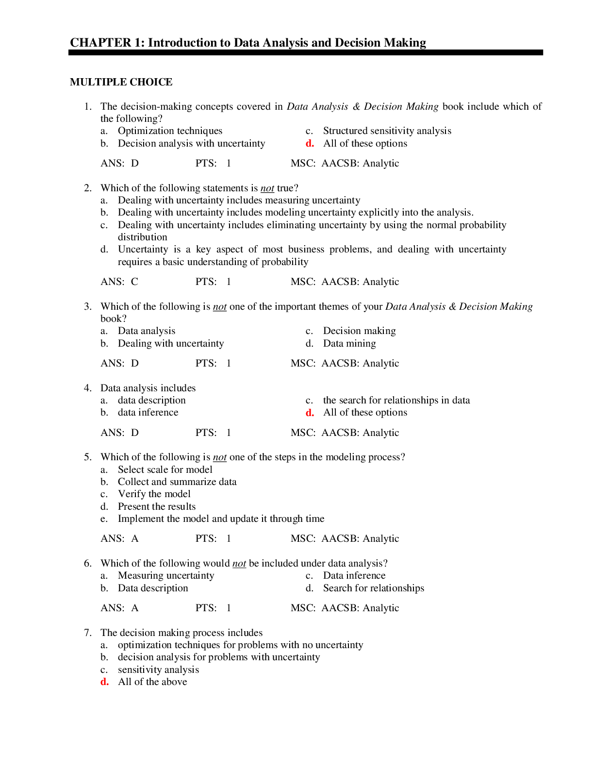
Reviews( 0 )
Document information
Connected school, study & course
About the document
Uploaded On
Nov 04, 2019
Number of pages
82
Written in

Additional information
This document has been written for:
Uploaded
Nov 04, 2019
Downloads
0
Views
286

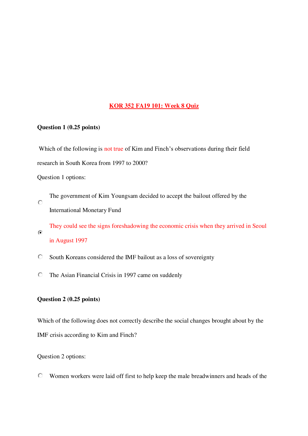
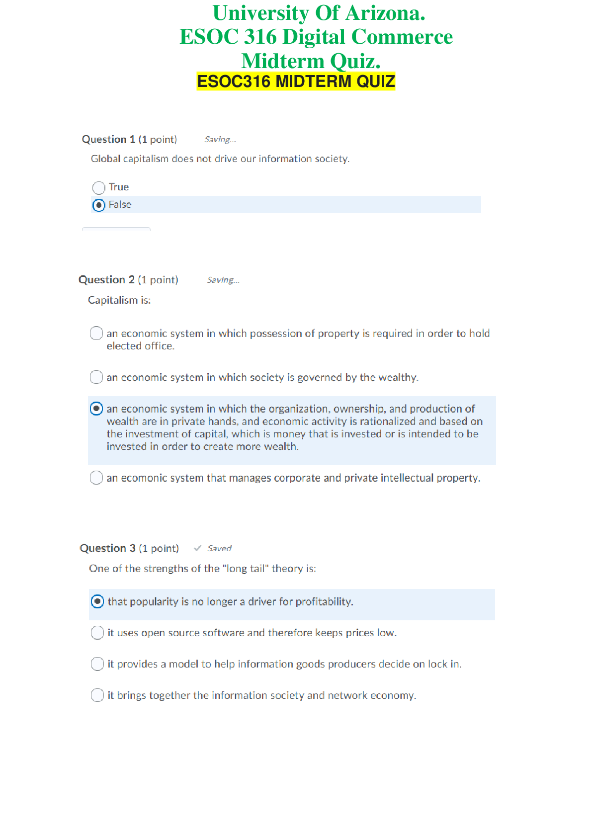

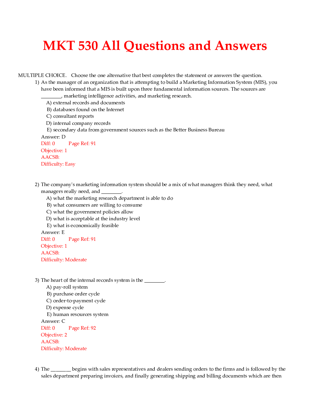
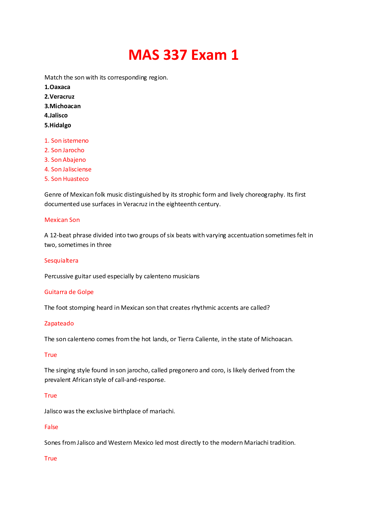


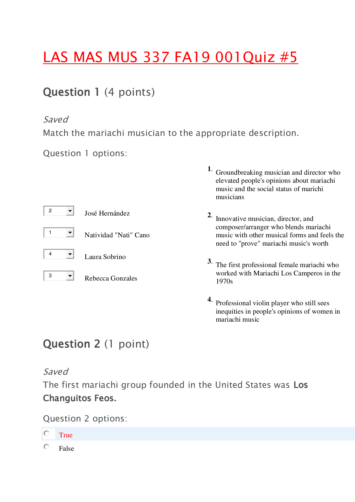

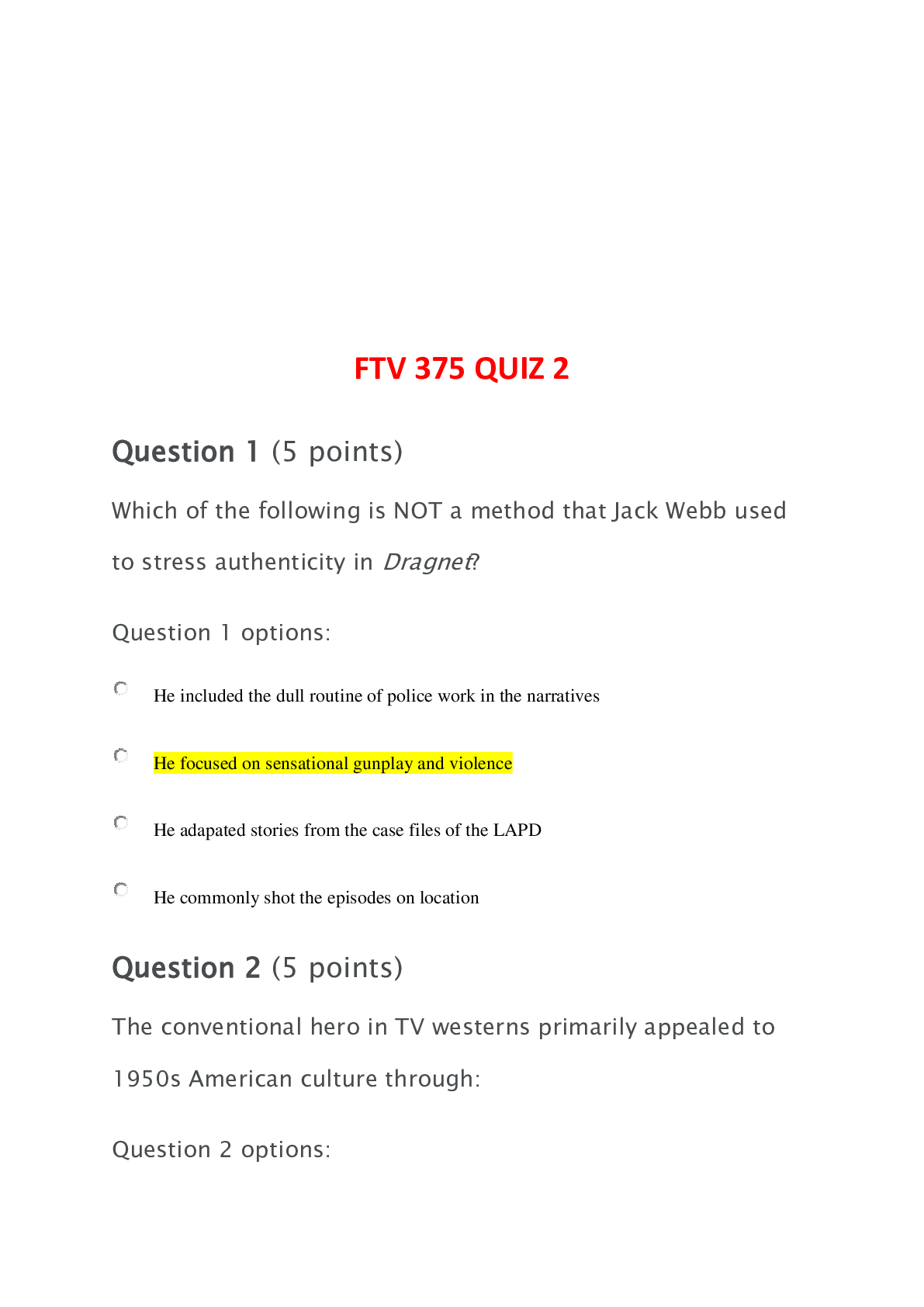
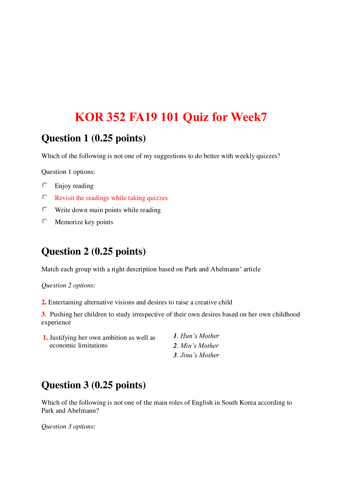
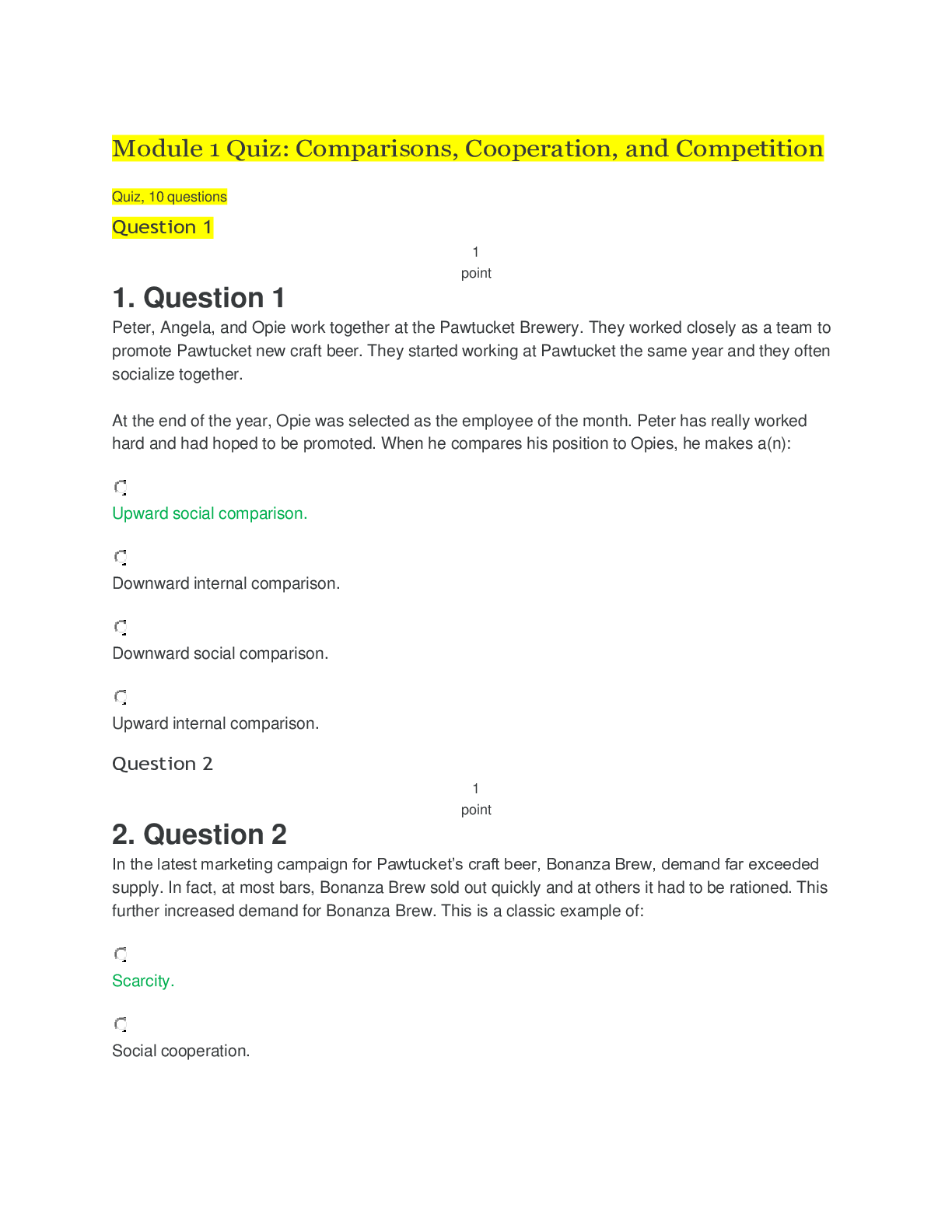
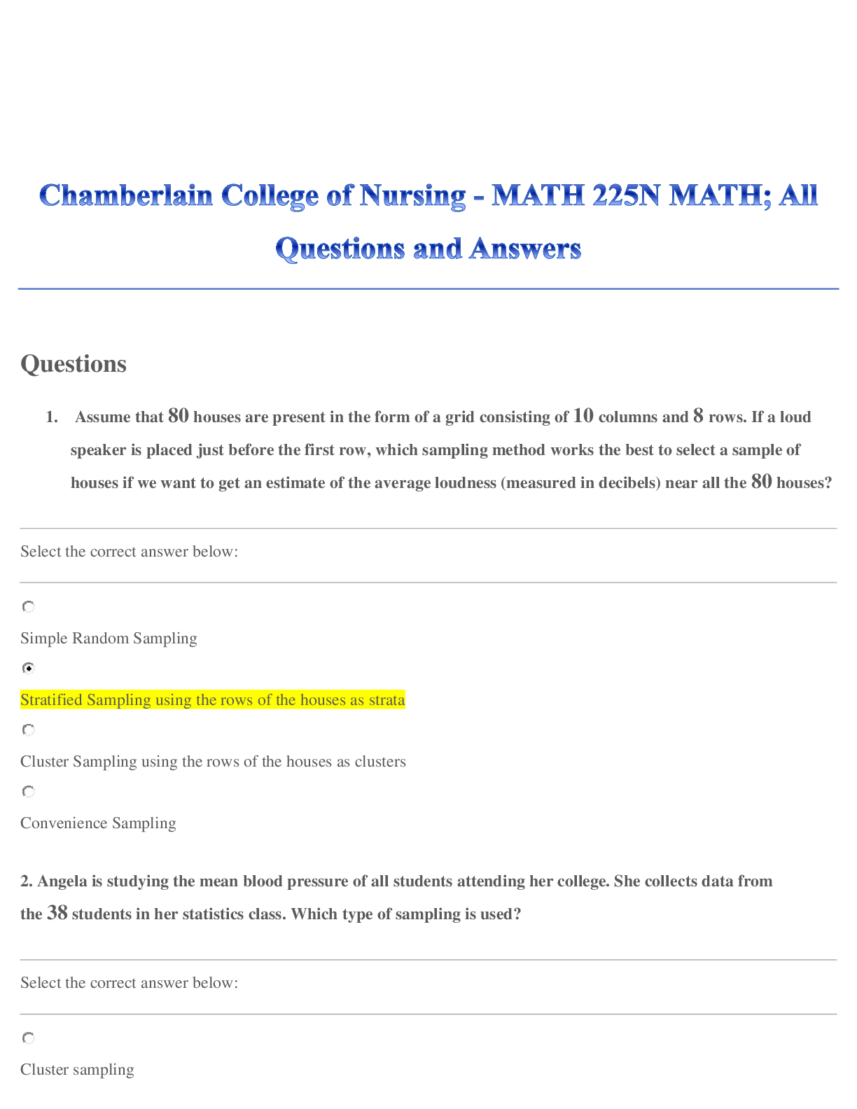


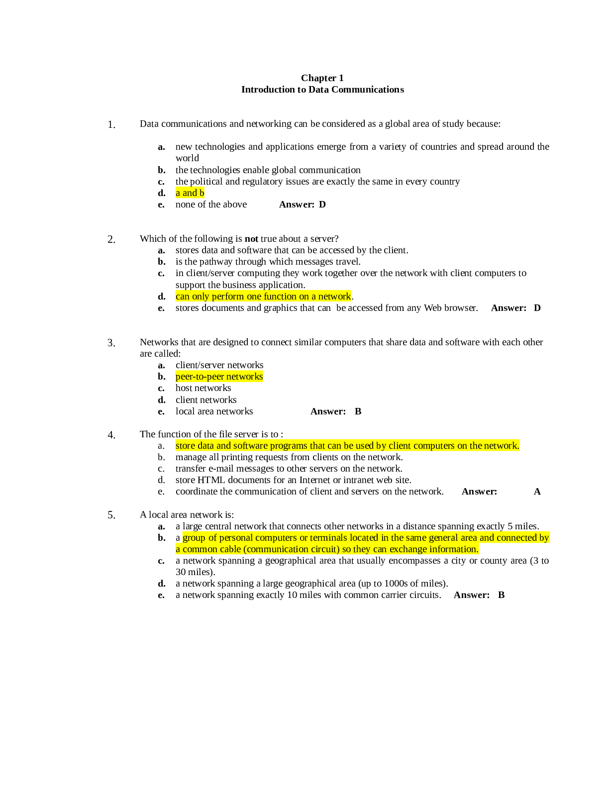

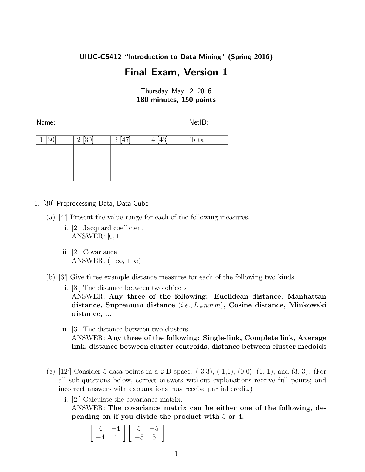


.png)
.png)

.png)