STAT 200 Stat 200 Week 6 Homework Question And Answers( Rated A)

Document Content and Description Below

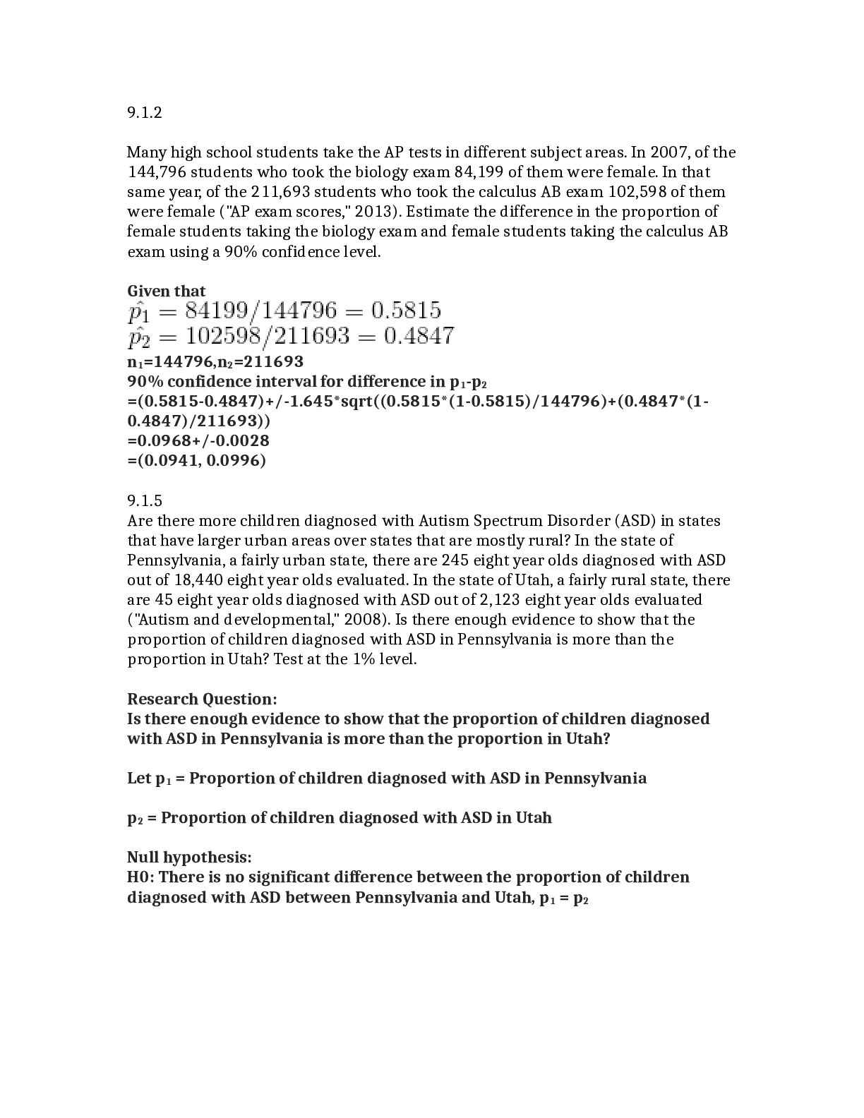
STAT 200 Stat 200 Week 6 Homework Question And Answers 9.1.2 Many high school students take the AP tests in different subject areas. In 2007, of the 144,796 students who took the biology exam 84,1... 99 of them were female. In that same year, of the 211,693 students who took the calculus AB exam 102,598 of them were female ("AP exam scores," 2013). Estimate the difference in the proportion of female students taking the biology exam and female students taking the calculus AB exam using a 90% confidence level. Given that n1=144796,n2=211693 90% confidence interval for difference in p1-p2 =(0.5815-0.4847)+/-1.645*sqrt((0.5815*(1-0.5815)/144796)+(0.4847*(1-0.4847)/211693)) =0.0968+/-0.0028 =(0.0941, 0.0996) 9.1.5 Are there more children diagnosed with Autism Spectrum Disorder (ASD) in states that have larger urban areas over states that are mostly rural? In the state of Pennsylvania, a fairly urban state, there are 245 eight year olds diagnosed with ASD out of 18,440 eight year olds evaluated. In the state of Utah, a fairly rural state, there are 45 eight year olds diagnosed with ASD out of 2,123 eight year olds evaluated ("Autism and developmental," 2008). Is there enough evidence to show that the proportion of children diagnosed with ASD in Pennsylvania is more than the proportion in Utah? Test at the 1% level. Research Question: Is there enough evidence to show that the proportion of children diagnosed with ASD in Pennsylvania is more than the proportion in Utah? Let p1 = Proportion of children diagnosed with ASD in Pennsylvania p2 = Proportion of children diagnosed with ASD in Utah Null hypothesis: H0: There is no significant difference between the proportion of children diagnosed with ASD between Pennsylvania and Utah, p1 = p2 Alternative hypothesis: H1: The proportion of children diagnosed with ASD in Pennsylvania is more than the porportion of children diagnosed with ASD in Utah, p1 > p2 Level of significance: Critical Region: Since, the alternative hypothesis is testing on the one-side(researcher is interseted if proportion in one group is more than the other) the hypothesis is tested at one tail. Therefore, form the standard normal table for 1% level of significance the Z-value is given as 2.33. Therefore, the null hypothesis will be rejected if the Z-test statistic is more than 2.33 Test statistic: Where p1 = Proportion of children diagnosed with ASD in Pennsylvania = 245/18440 = 0.0133 p2 = Proportion of children diagnosed with ASD in Utah = 45/2123 = 0.0212 n1 = Number of children in Pennsylvania = 18440 n2 = Number of children in Utah = 2123 x1 = Number of Children diagnosed with ASD in Pennsylvania = 245 x2 = Number of Children diagnosed with ASD in Utah = 45 Therefore, Inference: Since the calculated Z-test staitistic value of -2.9259 is lesser than the Z-critical value of 2.33, we will not reject the null hypothesis. Conclusion: There is no enough evidence to show that the proportion of children diagnosed with ASD in Pennsylvania is more than the proportion in Utah. 9.2.3 All Fresh Seafood is a wholesale fish company based on the east coast of the U.S. Catalina Offshore Products is a wholesale fish company based on the west coast of the U.S. Table #9.2.5 contains prices from both companies for specific fish types ("Seafood online," 2013) ("Buy sushi grade," 2013). Do the data provide enough evidence to show that a west coast fish wholesaler is more expensive than an east coast wholesaler? Test at the 5% level. Here, we use two sample t test to compare means. Let x = all fresh seafood prices & y = Catalina offshore products prices. For comparing two means, the basic null hypothesis is that the means are equal, ?0: ?1 = ?2 (i.e. the prices of both wholeseller are same) with the common alternative hypotheses, ?1: ?1 ≠ ?2 (i.e. the prices of both wholeseller are not same) Significance Level: α = 0.05 Degrees of freedom equal df = n1 + n2 −2 here n1 = n2 = 9, so df = 16 The test statistic is: where & and From the table & & if all the value are put in test statistic t , we get The tabulated value of t0.05 16 df (two tail test) = 2.4729 Since tcal < ttab, we accept the hypothesis and we can conclude that the prices of both wholesalers are the same. 9.2.6 The British Department of Transportation studied to see if people avoid driving on Friday the 13th. They did a traffic count on a Friday and then again on a Friday the 13th at the same two locations ("Friday the 13th," 2013). The data for each location on the two different dates is in table #9.2.6. Estimate the mean difference in traffic count between the 6th and the 13th using a 90% level. 9.3.1 The income of males in each state of the United States, including the District of Columbia and Puerto Rico, are given in table #9.3.3, and the income of females is given in table #9.3.4 ("Median income of," 2013). Is there enough evidence to show that the mean income of males is more than of females? Test at the 1% level. As we can see that the p value is less than 0.01 So, at 1% level of significance we conclude that there is enough evidence to support the claim that mean income of males is greater than income of females Explanation: R code: library(stringr) #Define x as the income of males x=c( 42951, 52379,42544,37488,49281, 50987,60705, 50411, 66760, 40951 ,43902 ,45494, 41528, 50746, 45183, 43624, 43993, 41612, 46313 ,43944 ,56708 ,60264 ,50053 ,50580 ,40202, 43146, 41635, 42182 ,41803, 53033, 60568, 41037, 50388, 41950, 44660, 46176, 41420, 45976, 47956 ,22529, 48842, 41464 ,40285 ,41309, 43160, 47573 ,44057, 52805, 53046, 42125, 46214 ,51630) numbers="31862 40550 36048 30752 41817 40236 47476 40500 60332 33823 35438 37242 31238 39150 34023 33745 33269 32684 31844 34599 48748 46185 36931 40416 29548 33865 31067 33424 35484 41021 47155 32316 42113 33459 32462 35746 31274 36027 37089 22117 41412 31330 31329 33184 35301 32843 38177 40969 40993 29688 35890 34381" #Define y as the income of females y=as.numeric(unlist(str_extract_all(numbers, "[\\.0-9e-]+"))) #Find the difference d=x-y #T test on the difference t.test(x,y,mu=0,alternative = c("greater"),var.equal = FALSE,conf.level=0.99) 9.3.3 A study was conducted that measured the total brain volume (TBV) (in mm3 ) of patients that had schizophrenia and patients that are considered normal. Table #9.3.5 contains the TBV of the normal patients and table #9.3.6 contains the TBV of schizophrenia patients ("SOCR data oct2009," 2013). Is there enough evidence to show that the patients with schizophrenia have less TBV on average than a patient that is considered normal? Test at the 10% level. 9.3.4 A study was conducted that measured the total brain volume (TBV) (in mm3 ) of patients that had schizophrenia and patients that are considered normal. Table #9.3.5 contains the TBV of the normal patients and table #9.3.6 contains the TBV of schizophrenia patients ("SOCR data oct2009," 2013). Compute a 90% confidence interval for the difference in TBV of normal patients and patients with Schizophrenia. SE( - )=sqrt(σ12/n1+σ22/n2)=31718 (1-alpha)*100% confidence interval for population mean difference= =sample mean difference ±z(alpha/2)*SE( - ) 90% confidence =(1463339-1445132)±z(0.05/2)*31718=18207 ±1.645*31718=18207 ±52176 =(-33969, 70383) x y n= 32 30 mean= 1463339 1445132 var= = 15247910906 28384048331 va/n= /n= 476497216 946134944 9.3.8 The number of cell phones per 100 residents in countries in Europe is given in table #9.3.9 for the year 2010. The number of cell phones per 100 residents in countries of the Americas is given in table #9.3.10 also for the year 2010 ("Population reference bureau," 2013). Find the 98% confidence interval for the different in mean number of cell phones per 100 residents in Europe and the Americas. # of cell phones per 100 European residents Mean = 108.151 Standard Deviation+ 29.965 # of cell phones per 100 American residents Mean = 87.205 Standard Deviation = 35.155 For Residents in Europe: For Residents in America: At =0.02, The critical value, = 2.33 98% confidence interval for the difference in the mean number of cell phone per 100 residents in Europe and America 11.3.2 Levi-Strauss Co manufactures clothing. The quality control department measures weekly values of different suppliers for the percentage difference of waste between the layout on the computer and the actual waste when the clothing is made (called run-up). The data is in table #11.3.3, and there are some negative values because sometimes the supplier is able to layout the pattern better than the computer ("Waste run up," 2013). Do the data show that there is a difference between some of the suppliers? Test at the 1% level. 11.3.4 [Show More]

Last updated: 1 year ago

Preview 1 out of 12 pages