Harvard University FIN 090 Assessment Review - Corporate Finance Institute. Advanced Excel Formulas Course.

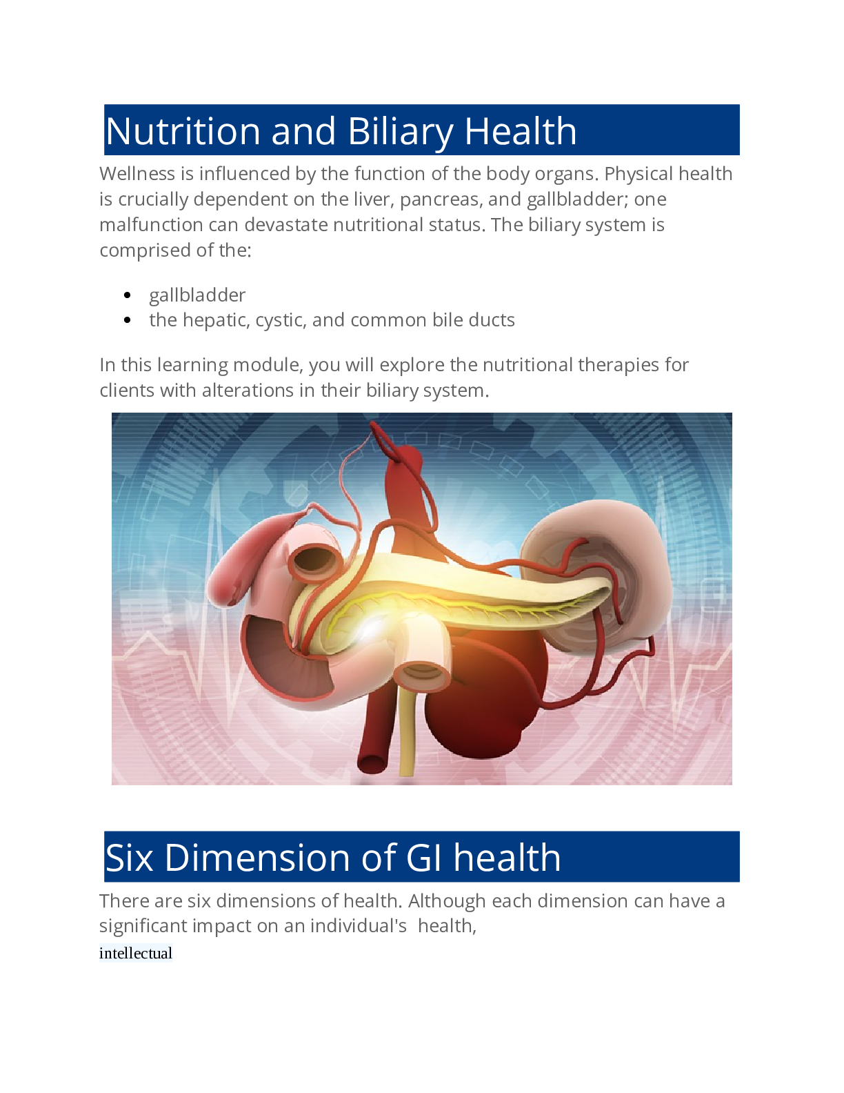
Document Content and Description Below

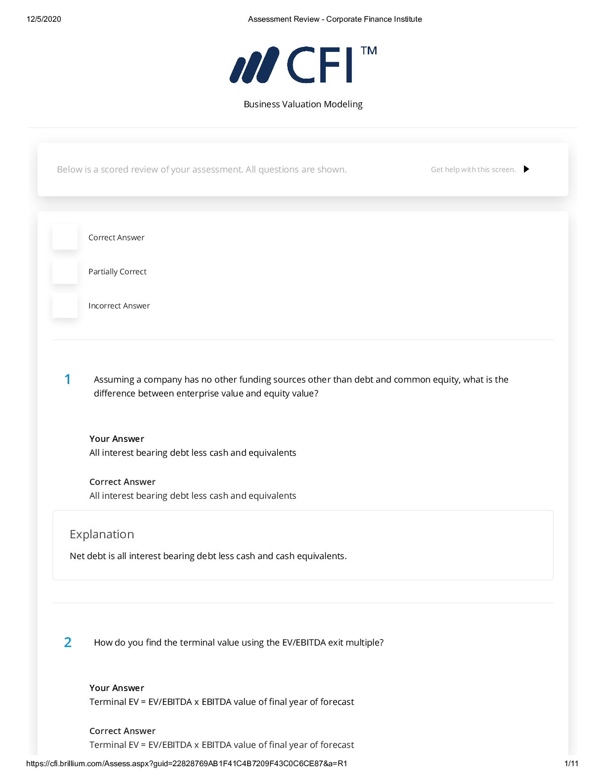
2020 Assessment Review - Corporate Finance Institute Advanced Excel Formulas Course 1 To return the value of the cell D8, the formula should be =OFFSET(A1, 1. , 2. ). A1 needs to move 7 rows down... and 3 columns to the right to reach D8. 2 To set up scenarios, you need to Òrst use ______ to set up a list, then ______ to set up the reference cell. Last you need to use ______ to set up the cells that display the output results from the scenario. 3 The 1. function calculates the repayment for a loan; the 2. function calculates the interest portion of the loan repayment. 4 Based on the image above, the dynamic formula that Ònds the XIRR of the 6th period would be: (must use cell B1 to make formula dynamic) =XIRR(B4:OFFSET(B4,0,_____),B3:OFFSET(B3,0,_____)) and the output would be _____ %. 5 The formula = INDEX(B2:F6,MATCH(“4x”,______,0),MATCH(“3x”,______,0)) would give the result of the cell with the red box. 6 =R1 4/9 Use goal seek to answer this question. All else equals, to have a net income of 20,000, the COGS margin percentage must be ______, and the gross proÒt must be ______. 7 The formula in the cell above would yield the result: 1. . 8 12/22/2020 Assessment Review - Corporate Finance Institute https://cfi.brillium.com/Assess.aspx?guid=A54F589B4EDC49108A78461ABC25433E&a=R1 5/9 The output of this function is: 1. =INDIRECT(MID(CELL("address",C3),2,1)&CELL("row",D6)) 9 The formula =MID("ABCDEFGHI",3,4) would yield the result: 1. . 10 The output of this function is: =IF(AND(C6>B7,OR(E1*A4=E4,D5<B10)),"TRUE","FALSE") 11 Pivot Table - Data.xlsx Please download and open the attached Òle. Round your answers to whole numbers, without the dollar symbol. Hats generated 1. total in revenue, and pants generated 2. in revenue through Instagram. Shorts generated on average 3. in revenue through AdWords. 4. (product) costed the most in shipping costs and 5. (channel) costed the most in marketing cost. Y A 12 Pivot Table - Data.xlsx Please download and open the attached Òle. Insert a Pivot Table, slicer, and timeline to answer the following questions. Round your answers to whole numbers, without the dollar symbol. For the Òrst 5 days, the total revenue generated through Facebook and Instagram is 1. . From Jan 4th to 6th, the revenue generated through non-social media channels (AdWords and Email) totals to 2. . 13 When creating a stacked chart to portray the breakdown of the income statement, the following item is not included:. 14 According to the lecture video on building dynamic charts, which of the following Excel functions are used in the "Refers to:" formula in Name Manager? Explanation We used the OFFSET and COUNT functions to build the formula in Name Manager in order to create dynamic charts. 15 The combo box (form control) option in macros can be used to substitute for ___ when doing scenario analysis. [Show More]

Last updated: 1 year ago

Preview 1 out of 9 pages