COMPSCI Final Cheat Sheet - SEARCH MDP II CSP II Iterative

Document Content and Description Below

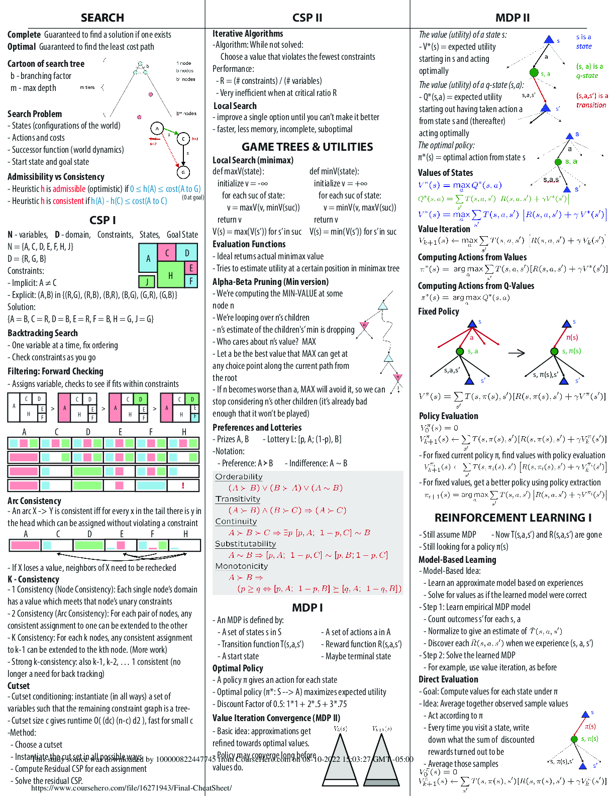
University of California, Berkeley COMPSCI 188 Final CheatSheet SEARCH Cartoon of search tree b - branching factor m - max depth Search Problem - Heuristic h is admissible (optimistic) if 0 ≤... h(A) ≤ cost(A to G) - Heuristic h is consistent if h(A) - h(C) ≤ cost(A to C) - States (congurations of the world) - Actions and costs - Successor function (world dynamics) - Start state and goal state Admissibility vs Consistency CSP I A H C D E F Complete Guaranteed to nd a solution if one exists Optimal Guaranteed to nd the least cost path J - One variable at a time, x ordering - Check constraints as you go Backtracking Search A C D E F H Filtering: Forward Checking ! - Assigns variable, checks to see if ts within constraints Arc Consistency - An arc X -> Y is consistent i for every x in the tail there is y in the head which can be assigned without violating a constraint A C -Algorithm: While not solved: Choose a value that violates the fewest constraints Performance: - R = (# constraints) / (# variables) - Very inecient when at critical ratio R D E F H - Cutset conditioning: instantiate (in all ways) a set of variables such that the remaining constraint graph is a tree- - Cutset size c gives runtime O( (dc) (n-c) d2 ), fast for small c -Method: - Choose a cutset - Instantiate the cut set in all possible ways - Compute Residual CSP for each assignment - Solve the residual CSP. - If X loses a value, neighbors of X need to be rechecked - 1 Consistency (Node Consistency): Each single node’s domain has a value which meets that node’s unary constraints - 2 Consistency (Arc Consistency): For each pair of nodes, any consistent assignment to one can be extended to the other - K Consistency: For each k nodes, any consistent assignment to k-1 can be extended to the kth node. (More work) - Strong k-consistency: also k-1, k-2, … 1 consistent (no longer a need for back tracking) K - Consistency Cutset CSP II - improve a single option until you can’t make it better - faster, less memory, incomplete, suboptimal Iterative Algorithms def minV(state): initialize v = +∞ for each suc of state: v = minV(v, maxV(suc)) return v V(s) = min(V(s’)) for s’ in suc Local Search def maxV(state): initialize v = -∞ for each suc of state: v = maxV(v, minV(suc)) return v V(s) = max(V(s’)) for s’ in suc GAME TREES & UTILITIES Evaluation Functions - We’re computing the MIN-VALUE at some node n - We’re looping over n’s children - n’s estimate of the children's’ min is dropping - Who cares about n’s value? MAX - Let a be the best value that MAX can get at any choice point along the current path from the root - Ideal returns actual minimax value - Tries to estimate utility at a certain position in minimax tree Local Search (minimax) Alpha-Beta Pruning (Min version) - An MDP is dened by: - A set of states s in S - A set of actions a in A - Transition function T(s,a,s’) - Reward function R(s,a,s’) - A start state - Maybe terminal state - Prizes A, B - Lottery L: [p, A; (1-p), B] -Notation: - Preference: A B - Indierence: A ~ B Preferences and Lotteries - If n becomes worse than a, MAX will avoid it, so we can stop considering n’s other children (it’s already bad enough that it won’t be played) - A policy π gives an action for each state - Optimal policy (π*: S --> A) maximizes expected utility - Discount Factor of 0.5: 1*1 + 2*.5 + 3*.75 Optimal Policy MDP I MDP II The value (utility) of a state s: - V*(s) = expected utility starting in s and acting optimally The value (utility) of a q-state (s,a): - Q*(s,a) = expected utility starting out having taken action a from state s and (thereafter) acting optimally The optimal policy: π*(s) = optimal action from state s Values of States Value Iteration Value Iteration Convergence (MDP II) - Basic idea: approximations get rened towards optimal values. - Policy may converge long before values do. Computing Actions from Values Computing Actions from Q-Values Fixed Policy Policy Evaluation - For xed current policy π, nd values with policy evaluation - Still assume MDP - Now T(s,a,s’) and R(s,a,s’) are gone - Still looking for a policy π(s) - For xed values, get a better policy using policy extraction REINFORCEMENT LEARNING I Model-Based Learning - Model-Based Idea: - Learn an approximate model based on experiences - Solve for values as if the learned model were correct - Step 1: Learn empirical MDP model - Count outcomes s’ for each s, a - Normalize to give an estimate of - Discover each when we experience (s, a, s’) - Step 2: Solve the learned MDP - For example, use value iteration, as before Direct Evaluation - Goal: Compute values for each state under π - Idea: Average together observed sample values - Act according to π - Every time you visit a state, write down what the sum of discounted rewards turned out to be - Average those samples [Show More]

Last updated: 1 week ago

Preview 1 out of 4 pages