University of Maryland - STAT 200; Week 7 Homework Problems, Already Graded A.

Document Content and Description Below

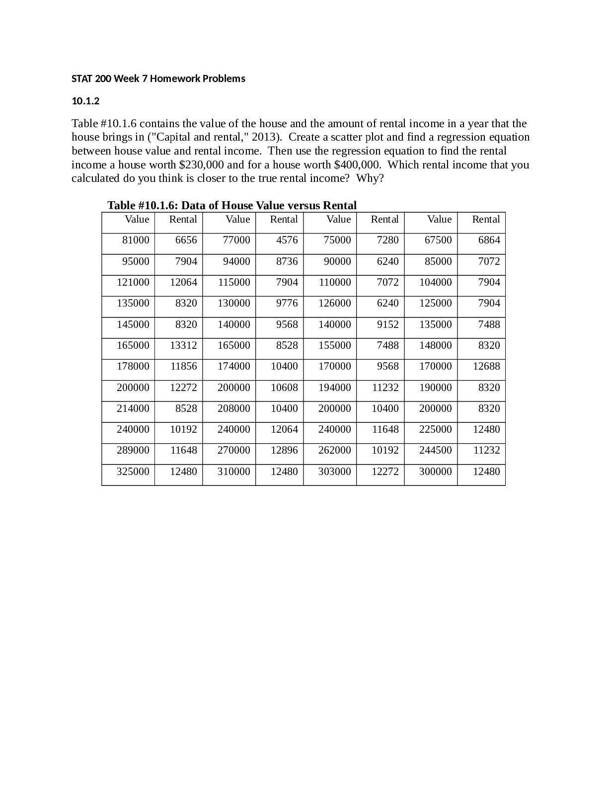
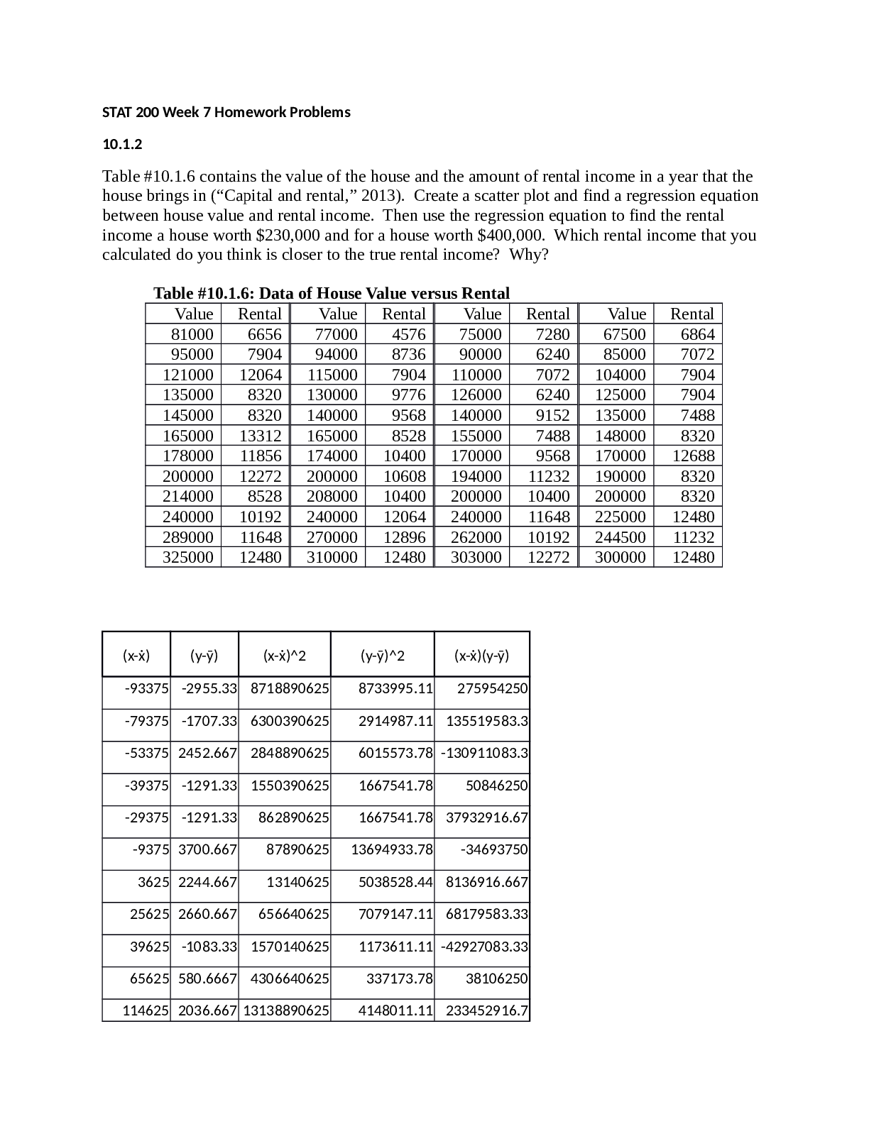
STAT 200 Week 7 Homework Problems 10.1.2 Table #10.1.6 contains the value of the house and the amount of rental income in a year that the house brings in (“Capital and rental,” 2013). Create a ... scatter plot and find a regression equation between house value and rental income. Then use the regression equation to find the rental income a house worth $230,000 and for a house worth $400,000. Which rental income that you calculated do you think is closer to the true rental income? Why? Table #10.1.6: Data of House Value versus Rental Value Rental Value Rental Value Rental Value Rental 81000 6656 77000 4576 75000 7280 67500 6864 95000 7904 94000 8736 90000 6240 85000 7072 121000 12064 115000 7904 110000 7072 104000 7904 135000 8320 130000 9776 126000 6240 125000 7904 145000 8320 140000 9568 140000 9152 135000 7488 165000 13312 165000 8528 155000 7488 148000 8320 178000 11856 174000 10400 170000 9568 170000 12688 200000 12272 200000 10608 194000 11232 190000 8320 214000 8528 208000 10400 200000 10400 200000 8320 240000 10192 240000 12064 240000 11648 225000 12480 289000 11648 270000 12896 262000 10192 244500 11232 325000 12480 310000 12480 303000 12272 300000 12480 (x-ẋ) (y-ӯ) (x-ẋ)^2 (y-ӯ)^2 (x-ẋ)(y-ӯ) -93375 -2955.33 8718890625 8733995.11 275954250 -79375 -1707.33 6300390625 2914987.11 135519583.3 -53375 2452.667 2848890625 6015573.78 -130911083.3 -39375 -1291.33 1550390625 1667541.78 50846250 -29375 -1291.33 862890625 1667541.78 37932916.67 -9375 3700.667 87890625 13694933.78 -34693750 3625 2244.667 13140625 5038528.44 8136916.667 25625 2660.667 656640625 7079147.11 68179583.33 39625 -1083.33 1570140625 1173611.11 -42927083.33 65625 580.6667 4306640625 337173.78 38106250 114625 2036.667 13138890625 4148011.11 233452916.7 150625 2868.667 22687890625 8229248.44 432092916.7 -97375 -5035.33 9481890625 25354581.78 490315583.3 -80375 -875.333 6460140625 766208.44 70354916.67 -59375 -1707.33 3525390625 2914987.11 101372916.7 -44375 164.6667 1969140625 27115.11 -7307083.333 -34375 -43.3333 1181640625 1877.78 1489583.333 -9375 -1083.33 87890625 1173611.11 10156250 -375 788.6667 140625 621995.11 -295750 25625 996.6667 656640625 993344.44 25539583.33 33625 788.6667 1130640625 621995.11 26518916.67 65625 2452.667 4306640625 6015573.78 160956250 95625 3284.667 9144140625 10789035.11 314096250 135625 2868.667 18394140625 8229248.44 389062916.7 -99375 -2331.33 9875390625 5435115.11 231676250 -84375 -3371.33 7119140625 11365888.44 284456250 -64375 -2539.33 4144140625 6448213.78 163469583.3 -48375 -3371.33 2340140625 11365888.44 163088250 -34375 -459.333 1181640625 210987.11 15789583.33 -19375 -2123.33 375390625 4508544.44 41139583.33 -4375 -43.3333 19140625 1877.78 189583.3333 19625 1620.667 385140625 2626560.44 31805583.33 25625 788.6667 656640625 621995.11 20209583.33 65625 2036.667 4306640625 4148011.11 133656250 87625 580.6667 7678140625 337173.78 50880916.67 128625 2660.667 16544390625 7079147.11 342228250 -106875 -2747.33 11422265625 7547840.44 293621250 -89375 -2539.33 7987890625 6448213.78 226952916.7 -70375 -1707.33 4952640625 2914987.11 120153583.3 -49375 -1707.33 2437890625 2914987.11 84299583.33 -39375 -2123.33 1550390625 4508544.44 83606250 -26375 -1291.33 695640625 1667541.78 34058916.67 -4375 3076.667 19140625 9465877.78 -13460416.67 15625 -1291.33 244140625 1667541.78 -20177083.33 25625 -1291.33 656640625 1667541.78 -33090416.67 50625 2868.667 2562890625 8229248.44 145226250 70125 1620.667 4917515625 2626560.44 113649250 125625 2868.667 15781640625 8229248.44 360376250 2.26936E+11 230247402.67 5527756000 (x-ẋ) (y-ӯ) SSx SSy SSxy 50000 100000 150000 200000 250000 300000 350000 0 2000 4000 6000 8000 10000 12000 14000 Scatter Plot Value Rental Slope = b= SSxy SSx y-intercept=a=ӯ-bx Regression Equation: ӯ=5363.86+0.0244x Ӯ=5363.89+ (0.0244*230,000)= $10,994.79 When the house value is $230,000, the predicted rental amount is $10,994.79 a month. Ӯ=5363.89+ (0.0244*230,000)= $15,156.78 When the house value is $400,000, the predicted rental amount is $15,156.78 a month. I think that the rental income that is closer to the true rental income is when the house value is $230,000, because the rental value is closer to the average of the total rental income. 10.1.4 The World Bank collected data on the percentage of GDP that a country spends on health expenditures (“Health expenditure,” 2013) and also the percentage of women receiving prenatal care (“Pregnant woman receiving,” 2013). The data for the countries where this information are available for the year 2011 is in table #10.1.8. Create a scatter plot of the data and find a regression equation between percentage spent on health expenditure and the percentage of women receiving prenatal care. Then use the regression equation to find the percent of women receiving prenatal care for a country that spends 5.0% of GDP on health expenditure and for a country that spends 12.0% of GDP. Which prenatal care percentage that you calculated do you think is closer to the true percentage? Why? 3 4 5 6 7 8 9 10 11 0 20 40 60 80 100 120 Scatter Plot Health Expenditure Parental Care Table #10.1.8: Data of Health Expenditure versus Prenatal Care Health Expenditur e (% of GDP) Prenatal Care (%) 9.6 47.9 slope 0.0244 y-intercept 5363.86 Regression Equation ӯ=5363.86+0.0244x 3.7 54.6 5.2 93.7 5.2 84.7 10.0 100.0 4.7 42.5 4.8 96.4 6.0 77.1 5.4 58.3 4.8 95.4 4.1 78.0 6.0 93.3 9.5 93.3 6.8 93.7 6.1 89.8 Slope = b= SSxy SSx y- intercept=a=ӯ-bx Regression Equation: ӯ=69.7394+1.6606x Ӯ=69.7394+ (1.6606*0.05)= 69.82% When the GDP is 5%, the predicted percent of women receiving prenatal care for a country is 69.82%. Ӯ=69.7394+ (1.6606*0.12)= 69.94% When the GDP is 12%, the predicted percent of women receiving prenatal care for a country is 69.94%. I think that prenatal care percentage that is closer to the true percentage is when the GDP is 12%. 10.2.2 Table #10.1.6 contains the value of the house and the amount of rental income in a year that the house brings in ("Capital and rental," 2013). Find the correlation coefficient and coefficient of determination and then interpret both. Table #10.1.6: Data of House Value versus Rental Value Rental Value Rental Value Rental Value Rental 81000 6656 77000 4576 75000 7280 67500 6864 95000 7904 94000 8736 90000 6240 85000 7072 121000 12064 115000 7904 110000 7072 104000 7904 135000 8320 130000 9776 126000 6240 125000 7904 145000 8320 140000 9568 140000 9152 135000 7488 slope 1.66060 y-intercept 69.7394 Regression Equation ӯ=69.7394+1.6606x 165000 13312 165000 8528 155000 7488 148000 8320 178000 11856 174000 10400 170000 9568 170000 12688 200000 12272 200000 [Show More]

Last updated: 1 year ago

Preview 1 out of 13 pages