STAT 200 - Homework 5 Solutions Question And Answers( Rated A)

Document Content and Description Below

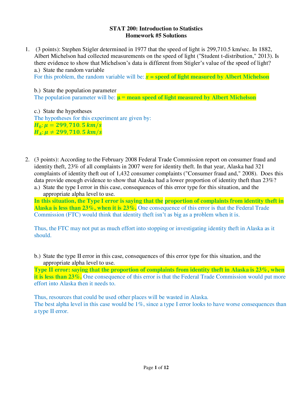
Page 1 of 12 STAT 200: Introduction to Statistics Homework #5 Solutions 1. (3 points): Stephen Stigler determined in 1977 that the speed of light is 299,710.5 km/sec. In 1882, Albert Michelson had... collected measurements on the speed of light ("Student t-distribution," 2013). Is there evidence to show that Michelson’s data is different from Stigler’s value of the speed of light? a.) State the random variable For this problem, the random variable will be: x = speed of light measured by Albert Michelson b.) State the population parameter The population parameter will be: μ = mean speed of light measured by Albert Michelson c.) State the hypotheses The hypotheses for this experiment are given by: ??: ? = ???, ???. ? ??/? ??: ? ≠ ???, ???. ? ??/? 2. (3 points): According to the February 2008 Federal Trade Commission report on consumer fraud and identity theft, 23% of all complaints in 2007 were for identity theft. In that year, Alaska had 321 complaints of identity theft out of 1,432 consumer complaints ("Consumer fraud and," 2008). Does this data provide enough evidence to show that Alaska had a lower proportion of identity theft than 23%? a.) State the type I error in this case, consequences of this error type for this situation, and the appropriate alpha level to use. In this situation, the Type I error is saying that the proportion of complaints from identity theft in Alaska is less than 23%, when it is 23%. One consequence of this error is that the Federal Trade Commission (FTC) would think that identity theft isn’t as big as a problem when it is. Thus, the FTC may not put as much effort into stopping or investigating identity theft in Alaska as it should. b.) State the type II error in this case, consequences of this error type for this situation, and the appropriate alpha level to use. Type II error: saying that the proportion of complaints from identity theft in Alaska is 23%, when it is less than 23%. One consequence of this error is that the Federal Trade Commission would put more effort into Alaska then it needs to. Thus, resources that could be used other places will be wasted in Alaska. The best alpha level in this case would be 1%, since a type I error looks to have worse consequences than a type II error. Page 2 of 12 3. (3 points): According to the February 2008 Federal Trade Commission report on consumer fraud and identity theft, 23% of all complaints in 2007 were for identity theft. In that year, Alaska had 321 complaints of identity theft out of 1,432 consumer complaints ("Consumer fraud and," 2008). Does this data provide enough evidence to show that Alaska had a lower proportion of identity theft than 23%? Why or why not? Test at the 5% level. We should start by writing down what we know (which is always a great place to start): x = 321 n = 1432 p = 0.23 (or 23%) α = 0.05 To fully address this problem, we shoudl follow the six step process presented in the textbook. i.) State the random variable and the parameter in words. The random variable is given by: x = number of complaints from identity theft in Alaska The parameter of interest is given by: p = proportion of complaints from identity theft in Alaska ii.) State the null and alternative hypotheses and the level of significance The hypotheses for this experiment are given by: ?0: ? = 0.23 ??: ? < 0.23 The level of significance is α = 0.05. iii.) State and check the assumptions for a hypothesis test a) A simple random sample of the category of 1432 complaints of identity theft in Alaska was taken. The study says that the complaints were out of all complaints that year, but the year could have been chosen at random. This assumption may be met, but you can’t be sure. b) There are 1432 complaints in this sample. The reason for the complaint does not affect the next complaint. There are only two outcomes, either the complaint was for identity theft or it wasn’t. The chance that one complaint was for identity theft does not change. Thus the conditions for the binomial distribution are satisfied c) In this case p = 0.23 and n = 1432. np = 1432 * 0.23 = 329.36 ≥ 5 and nq = 1432 * (1 – 0.23) = 1102.64 ≥ 5. Thus, the sampling distribution for ?̂is a normal distribution; this means we will use a z-test. iv.) Find the sample statistic, test statistic, and p-value The sample proportion is given by: x = 321 n = 1432  ?̂= ? ? = 321 1432 = 0.2242 The test statistic is given by: ? = ?̂− ? √ ?? ? = 0.2242 − 0.23 √ 0.23(1 − 0.23) 1432 = −0.522 The p-value associated with this problem (going back to homework 4 for how to compute the p-value from a z-statistic) is given by: = NORM.S.DIST(z,cumulative) = NORM.S.DIST (-0.522, TRUE) = 0.2998 Page 3 of 12 v.) Conclusion Since the p-value is greater than the level of significance (i.e. [p-value = 0.2998] > [α = 0.05]), we fail to reject ??. vi.) Interpretation (do not skip this part! This is the “so what” of the entire hypothesis test). There is not enough evidence to show that the proportion of complaints due to identity theft in Alaska is less than 23%. 4. (3 points): In 2008, there were 507 children in Arizona out of 32,601 who were diagnosed with Autism Spectrum Disorder (ASD) ("Autism and developmental," 2008). Nationally 1 in 88 children are diagnosed with ASD ("CDC features -," 2013). Is there sufficient data to show that the incident of ASD is more in Arizona than nationally? Why or why not? Test at the 1% level. We should start by writing down what we know (which is always a great place to start): x = 507 n = 32,601 p = 1/88 = 0.0114 (or 1.14%) α = 0.01 To fully address this problem, we should follow the six step process presented in the textbook. i.) State the random variable and the parameter in words. The random variable is given by: x = number of children in Arizona in 2008 that were diagnosed with Autism Spectrum Disorder (ASD) The parameter of interest is given by: p = proportion of children in Arizona in 2008 that were diagnosed with Autism Spectrum Disorder (ASD) ii.) State the null and alternative hypotheses and the level of significance The hypotheses for this experiment are given by: ?0: ? = 1 88 = 0.0114 ??: ? > 1 88 = 0.0114 The level of significance is α = 0.01. iii.) State and check the assumptions for a hypothesis test a) A simple random sample of the 32,601 diagnoses of children was taken in 2008. The study was conducted by the CDC so this assumption is probably true. b) ii. There are 32,601 diagnoses in this sample. The diagnoses of one Arizona child doesn’t affect the opinion of the next one. There are only two outcomes, either the Arizona child has ASD or they do not. The chance that one Arizona child has ASD does not change. Thus the conditions for the binomial distribution are satisfied c) In this case p = 1 88 = 0.0114 and n = 32,601. np = 32601 * 1 88 = 370.47 ≥ 5 and nq = 32601 * (1 – 1 88 ) = 32,230.5 ≥ 5. Thus, the sampling distribution for ?̂is a normal distribution; this means we will use a z-test. Page 4 of 12 iv.) Find the sample statistic, test statistic, and p-value The sample proportion is given by: x = 507 n = 32,601  ?̂= ? ? = 507 32,601 = 0.0156 The test statistic is given by: ? = ?̂− ? √ ?? ? = 0.0156 − 0.0114 √ 0.0114(1 − 0.0114) 32601 = 7.134 The p-value associated with this problem (going back to homework 4 for how to compute the p-value from a z-statistic) is given by: =1 - NORM.S.DIST(z,cumulative) =1 - NORM.S.DIST (7.134, TRUE) = 4.866 * 10-13 v.) Conclusion Since the p-value is less than the level of significance (i.e. [p-value = 4.866 * 10-13] < [α = 0.01]), we reject ??. vi.) Interpretation (do not skip this part! This is the “so what” of the entire hypothesis test). There is enough evidence to show that the proportion of Arizona children in 2008 with ASD is more than the national proportion. 5. (3 points): The economic dynamism, which is the index of productive growth in dollars for countries that are designated by the World Bank as middle-income are in Table 1 ("SOCR data 2008," 2013). Countries that are considered high-income have a mean economic dynamism of 60.29. Does the data show that the mean economic dynamism of middle-income countries is less than the mean for high income countries? Why or why not? Test at the 5% level. 25.8057 37.4511 51.9150 43.6952 47.8506 43.7178 58.0767 41.1648 38.0793 37.7251 39.6553 42.0265 48.6159 43.8555 49.1361 61.9281 41.9543 44.9346 46.0521 48.3652 43.6252 50.9866 59.1724 39.6282 33.6074 21.6643 Table 1: Economic Dynamism of Middle Income Countries i.) State the random variable and the parameter in words. x = economic dynamism for a middle-income country μ = mean economic dynamism for middle-income countries ii.) State the null and alternative hypotheses and the level of significance ?0: ? = $60.29 ??: ? < $60.29 ? = 0.05 Page 5 of 12 iii.) State and check the assumptions for a hypothesis test a) A simple random sample of economic dynamism for 26 middle-income countries was taken. The problem doesn’t mention how the sample was taken. So this requirement may not have been met. b) The population of the economic dynamism for all middle-income countries is normally distributed or the sample size is 30 or more. The sample size is 26. The histogram looks somewhat bell shaped, there is one outlier (but it is not far outside 1.5*IQR), and the normal probability plot does appear linear. Thus, this assumption is probably met (nothing is ever “perfect” in real life). Page 6 of 12 iv.) Find the sample statistic, test statistic, and p-value Sample mean and standard deviation: ?̅= $43.87 ? = $9.07 n = 26 Test Statistic: ? = ?̅− ? ? √? ⁄ = 43.87 − 60.29 9.07 √26 ⁄ = −9.228 p-value: To get the p-value from excel, we use the t.dist function: Syntax: T.DIST(x,deg_freedom, cumulative) The T.DIST function syntax has the following arguments: X Required. The numeric value at which to evaluate the distribution Deg_freedom Required. An integer indicating the number of degrees of freedom. Cumulative Required. A logical value that determines the form of the function. If cumulative is TRUE, T.DIST returns the cumulative distribution function; if FALSE, it returns the probability density function. The function to put into Excel is: =T.DIST(-9.228, 26-1, TRUE) = 7.900 * 10-10 v.) Conclusion Since the p-value is less than the significance level (i.e. 7.900 * 10-10 < 0.05), we reject ?? vi.) Interpretation There is enough evidence to show that the mean economic dynamism for a middle-income country is less than 60.29, the mean for high-income countries. -2.5 -2 -1.5 -1 -0.5 0 0.5 1 1.5 2 2.5 0.0000 10.0000 20.0000 30.0000 40.0000 50.0000 60.0000 70.0000 Normal Probability Plot for Economic Dynamism Page 7 of 12 6. (3 points): Maintaining your balance may get harder as you grow older. A study was conducted to see how steady the elderly is on their feet. They had the subjects stand on a force platform and have them react to a noise. The force platform then measured how much they swayed forward and backward, and the data is in table #7.3.10 ("Maintaining balance while," 2013). Does the data show that the elderly sway more than the mean forward sway of younger people, which is 18.125 mm? Why or why not? Test at the 1% level. 19 30 20 19 29 25 21 24 50 Table 2: Forward/backward Sway (in mm) of Elderly Subjects i.) State the random variable and the parameter in words. x = forward and backward sway of an elderly person μ = mean forward and backward sway of an elderly person ii.) State the null and alternative hypotheses and the level of significance ?0: ? = 18.125 ?? ??: ? > 18.125 ?? ? = 0.01 iii.) State and check the assumptions for a hypothesis test a) A simple random sample of the forward and backward sway of 9 elderly people was taken. The problem doesn’t mention how the sample was taken. So this requirement may not have been met. b) The population of the forward and backward sway of all elderly people is normally distributed. The histogram does not look bell shaped, there is one outlier, and the normal probability plot does not appear linear. Thus, this assumption may not be met. -2 -1 0 1 2 0 10 20 30 40 50 60 Normal Probabiltiy Plot for Sway Page 8 of 12 iv.) Find the sample statistic, test statistic, and p-value Sample mean and standard deviation: ?̅= 26.33 ?? ? = 9.77 ?? n = 9 Test Statistic: ? = ?̅− ? ? √? ⁄ = 26.33 − 18.125 9.77 √9 ⁄ = 2.5198 p-value: To get the p-value from excel, we use the t.dist function; however, we are looking for the area to the left (our alternative hypothesis is “greater than”), so we take 1 – the area to the left. In Excel: =1-T.DIST(2.5198, 9-1, TRUE) = 0.0179 v.) Conclusion Since the p-value is greater than the significance level (i.e. 0.0179 > 0.01), we fail to reject ?? vi.) Interpretation There is not quite enough evidence to show that the mean sway forward and backward of elderly people is more than 18.125 mm, the sway of younger people at the 0.01 (or 1%) level. However, if we increased our level of significance to 0.05 (the 5% level), we would conclude that the mean sway of elderly people is more than that of younger people. 7. (3 points): Suppose you compute a confidence interval with a sample size of 100. What will happen to the confidence interval if the sample size decreases to 80? A confidence interval will become wider if the sample size is decreased. 8. (3 points): In 2013, Gallup conducted a poll and found a 95% confidence interval of 0.52  p  0.60, where p is the proportion of Americans who believe it is the government’s responsibility for health care. Give the statistical interpretation. The proportion of Americans who believe it is the government’s responsibility for health care is between 52% and 60%. 9. (3 points): In 2008, there were 507 children in Arizona out of 32,601 who were diagnosed with Autism Spectrum Disorder (ASD) ("Autism and developmental," 2008). Find the proportion of ASD in Arizona with a confidence level of 99%. This is a confidence interval about a proportion. Thus, we will use the standard normal distribution. i.) State the random variable and the parameter in words. x = number of children in Arizona in 2008 that were diagnosed with Autism Spectrum Disorder (ASD) p = proportion of children in Arizona in 2008 that were diagnosed with Autism Spectrum Disorder (ASD) Page 9 of 12 ii.) State and check the assumptions a. A simple random sample of the 32,601 diagnoses of children was taken in 2008. The study was conducted by the CDC, so this assumption is probably true. b. There are 32,601 diagnoses in this sample. The diagnoses of one Arizona child doesn’t affect the opinion of the next one. There are only two outcomes, either the Arizona child has ASD or they do not. The chance that one Arizona child has ASD does not change. Thus, the conditions for the binomial distribution are satisfied c. In this case, ?̂= ? ? = 507 32,601 = 0.0156 and n = 32601. Thus, n?̂= 32601 * 507 32,601 = 507 ≥ 5 and n?̂ = 32601 * (32,601−507 32,601 ) = 32094 ≥ 5. Thus, the sampling distribution for ?̂is a normal distribution. iv.) Find the sample statistic and confidence interval The sample proportion is given by: x = 507 n = 32,601  ?̂= ? ? = 507 32,601 = 0.0156 Confidence Interval: First, we need to determine the value for ?? , the critical value where C = 1 – α If we use Table A.1 in the back of the Kozak textbook, we find this value is 2.575. Table A.1: Normal Critical Values for Confidence Levels Confidence Level, C Critical Value, zc 99% 2.575 98% 2.33 95% 1.96 90% 1.645 80% 1.28 You might actually want to know from where this value came, so here is how you can find it in Excel: Since we are looking at the 99% confidence interval, we have an area of 1 – 0.99 = 0.01 outside of our confidence interval; however, half is on both sides of the interval. Thus, it goes from 0.005 to 0.995. We can use the standard normal distribution for either value—just remember that we always want to use the positive value for ?? . The equation we use is: =NORM.S.INV(0.995) = 2.5758 (which is just a little different from the table above, but probably not enough to matter). Next, we need to compute the margin of error, given by: ? = ??√ ?̂?̂ ? = 2.5758√ (0.01555)(1 − 0.01555) 32601 = 0.0018 Page 10 of 12 The last step is to put this into the confidence interval equation: ?̂− ? < ? < ?̂+ ? 0.01555 − 0.0018 < ? < 0.01555 + 0.0018 0.01379 < ? < 0.01732 iv). Statistical Interpretation: There is a 99% chance that the interval ?. ????? < ? < ?. ????? contains the true proportion of children in Arizona in 2008 that were diagnosed with Autism Spectrum Disorder (ASD). v.) Real World Interpretation: The proportion of children in Arizona in 2008 that were diagnosed with Autism Spectrum Disorder (ASD) is between 0.01379 and 0.017321. 10. (3 points): The economic dynamism, which is the index of productive growth in dollars for countries that are designated by the World Bank as middle-income are in Table 1 ("SOCR data 2008," 2013). NOTE: this is the same data set from question 5. Compute a 95% confidence interval for the mean economic dynamism of middle-income countries. 25.8057 37.4511 51.9150 43.6952 47.8506 43.7178 58.0767 41.1648 38.0793 37.7251 39.6553 42.0265 48.6159 43.8555 49.1361 61.9281 41.9543 44.9346 46.0521 48.3652 43.6252 50.9866 59.1724 39.6282 33.6074 21.6643 Table 1: Economic Dynamism of Middle Income Countries This is a confidence interval about the mean, when the population mean is NOT known. Thus, we will use Student’s t distribution. i.) State the random variable and the parameter in words. x = economic dynamism for a middle-income country p = mean economic dynamism for middle-income countries ii.) State and check the assumptions a. A simple random sample of economic dynamism for 26 middle-income countries was taken. The problem doesn’t mention how the sample was taken. Thus, this assumption may not have been met. b. Recall from question 5: The population of the economic dynamism for all middle-income countries is normally distributed or the sample size is 30 or more. The sample size is 26. The histogram looks somewhat bell shaped, there is one outlier (but it is not far outside 1.5*IQR), and the normal probability plot does appear linear. Thus, this assumption is probably met (nothing is ever “perfect” in real life). iv.) Find the sample statistic and confidence interval Also from question 5: Sample mean and standard deviation: ?̅= $43.87 ? = $9.07 n = 26 Page 11 of 12 Confidence Interval: First, we need to determine the value for ?? , the critical value where C = 1 – α If we use Table A.2 in the back of the Kozak textbook, we look in the 95% column down to degrees of freedom of n – 1 = 26 – 1 = 25 and find the value of tc = 2.060. You might actually want to know from where this value came, so here is how you can find it in Excel: Since we are looking at the 95% confidence interval, we have an area of 1 – 0.95 = 0.05 outside of our confidence interval; however, half is on both sides of the interval. Thus, it goes from 0.025 to 0.975. Page 12 of 12 We can use the student t distribution for either value—just remember that we always want to use the positive value for ?? . The equation we use is: The Syntax for this equation is: T.INV(probability, deg_freedom) The T.INV function syntax has the following arguments: • Probability The probability associated with the Student's t-distribution in one tail. • Deg_freedom The number of degrees of freedom with which to characterize the distribution. Thus, for this problem, the equation is: “=T.INV( (1- 0.95)/2, 26-1)” = 2.0595 Excel also has an equation to compute a 2-tailed student t-distribution. NOTE: This obviously should only be applied to a 2-tailed test! The Syntax for this equation is: T.INV.2T(probability, deg_freedom) The T.INV.2T function syntax has the following arguments: • Probability The combined probability associated with the Student's t-distribution in the tails. • Deg_freedom The number of degrees of freedom with which to characterize the distribution. Thus, for this problem, the equation is: “=T.INV.2T(1-0.95, 26-1)” = 2.0595 Next, we need to compute the margin of error, given by: ? = ?? ? √? = 2.060 9.07 √36 = $3.66 The last step is to put this into the confidence interval equation: ?̂− ? < ? < ?̂+ ? 43.87 − 3.66 < ? < 43.87 + 3.66 40.21 < ? < 47.54 iv). Statistical Interpretation: There is a 95% chance that the interval ??. ?? < ? < ??. ?? contains the true mean economic dynamism for middle-income countries. v.) Real World Interpretation: The mean economic dynamism for middle-income countries is between $40.21 and $47.54. [Show More]

Last updated: 1 year ago

Preview 1 out of 12 pages